Binary Classification of Record Data (REKT Database) with Decision Trees
The purpose of this tab is to examine the performance of the Decision Tree Classifier on our cleaned record data gathered from the REKT Database API. and News APIs. If we recall, we conducted multiclass classification on the variable “scam_type” using Naive Bayes in R. For this tab, we shall code in Python and compare the results of the Naive Bayes classifier as well as a baseline random classifier to the results of the Decision Tree Classifier. Like SVM, we shall conduct hyperparameter tuning and try to achieve the lowest training and test errors for our Decision Tree Classifier.
Methods
Before we begin modeling our Decision Tree Classifier, we shall test the record data on a random classifier, which is a baseline model, and output its accuracy, precision, and recall values. We shall use sklearn’s train-test split function to divide the data into an 80-20 train-test split respectively. Next, we shall employ the Decision Tree Classifier and compare its initial and hyperparameter turned performance with each other and with the random classifier. While performing hyperparameter tuning, we shall use sklearn’s GridSearchCV(), like we did for the SVM tab, and change the max_depth, min_samples_leaf, and criterion values. Our goal is to try to achieve the best performing Decision Tree Classifier, which can outperform the Naive Bayes Classifier, which was coded in R.
Results
The cleaned REKT Database has 816 observations after pre-processing. If we recall, the original REKT Database had 3076 observations; however, to treat the heavy class imbalance present in the original data, about 1861 honeypots, 383 rugpulls, and 29 “other” scams were filtered out. Moreover, no key information, in terms of funds lost or source of the attack, was offered about these attacks in the observations that were eliminated. We are left with all those rows where funds lost != 0 and where all projects have some information to offer regarding the extent of the scam, helpful in predicting the scam type.
Recalling from the Naive Bayes tab, the initial Naive Bayes Classifier that was tested on the same record data outputted an accuracy of 60% on the test data and the discretized Naive Bayes Classifier outputted an accuracy of 72%. Our expectation is that the Decision Tree should perform better than the Naive Bayes Classifiers because the Decision Tree is a more complex and stronger algorithm than Naive Bayes. Indeed, we are proved correct, as the initial Decision Tree outputted a 100% on all metrics on the training data and a 62% accuracy on the test data. This indicated major overfitting on the training data and, hence, hyperparameter tuning was employed for the Decision Tree to generalize better on unseen data. After performing hyperparameter tuning, the accuracy on the test data was significantly higher at 76%, which means that the Decision Tree did outperform the Naive Bayes Classifier trained on discretized data. Therefore, hyperparameter tuning is an important step in the machine learning process and it opens insights on why and how a particular model performs when its parameters are dialed back and forth.
Loading Libraries and the Cleaned Record Data (REKT Database)
Code
import pandas as pdimport seaborn as sns import matplotlib.pyplot as pltfrom sklearn import treefrom IPython.display import Imageimport numpy as npfrom sklearn.metrics import accuracy_scorefrom sklearn.metrics import precision_scorefrom sklearn.metrics import recall_scorefrom sklearn.metrics import confusion_matrix, ConfusionMatrixDisplay, classification_reportimport warningswarnings.filterwarnings("ignore")
Code
# LOAD THE DATAFRAMEdf = pd.read_csv("../../data/Clean Data/REKT_Database_Clean_Classification.csv", index_col=[0])
Code
# Visualize first 5 rowsdf.head(5)
log_funds_lost
log_funds_returned
scamNetworks
month_of_attack
day_of_week_of_attack
day_of_year_of_attack
scam_type_grouped
1
15.319588
0.0
Ethereum
8
6
241
Exploit
2
10.603213
0.0
Avax
5
1
151
Exit Scam
3
15.420940
0.0
CEX
4
5
112
Exploit
4
13.504419
0.0
Binance
7
2
194
Exit Scam
5
9.798127
0.0
Fantom
5
5
134
Exploit
Code
# PRINT SHAPE
print("Data shape is: ", df.shape)
Data shape is: (816, 7)
Exploring the Pre-processed Data using Correlation Heat Maps and Pairplots
Scam type is the dependent variable, which contains 2 labels, Exit Scam (381 observations) and Exploit (435 observations). The independent variables are a mix of continuous, discrete, and text data. The independent continuous variables are log_funds_lost and log_funds_returned. The independent discrete variables are 3 datetime features, including month_of_attack, day_of_week_of_attack, and day_of_year_of_attack. The only string independent variable is scamNetworks, which denotes the token attached to the project that got scammed.
Code
# RUN THE FOLLOWING CODE TO SHOW THE HEAT-MAP FOR THE CORRELATION MATRIXcorr = df.corr();#print(corr) #COMPUTE CORRELATION OF FEATER MATRIXprint(corr.shape)sns.set_theme(style="white")f, ax = plt.subplots(figsize=(10, 5), dpi=150) # Set up the matplotlib figurecmap = sns.diverging_palette(230, 20, as_cmap=True) # Generate a custom diverging colormap# Draw the heatmap with the mask and correct aspect ratiosns.heatmap(corr, cmap=cmap, vmin=-1, vmax=1, center=0, square=True, linewidths=.5, cbar_kws={"shrink": .5})plt.xticks(rotation=45,fontsize=10)plt.show();# semi colon not needed
(5, 5)
Code
# GENERATING A SEABORN PAIRPLOT
sns.pairplot(df,hue="scam_type_grouped", diag_kind='kde')
<seaborn.axisgrid.PairGrid at 0x14b21d670>
Split the dataset into training and testing sets
Code
# MAKE DATA-FRAMES (or numpy arrays) (X,Y) WHERE Y="target" COLUMN and X="everything else"X = df.drop('scam_type_grouped', axis=1)y = df['scam_type_grouped']
Code
# PARTITION THE DATASET INTO TRAINING AND TEST SETSfrom sklearn.model_selection import train_test_splitx_train, x_test, y_train, y_test = train_test_split(X, y, random_state =1,test_size=0.2)
Code
# PRINT THE TYPE AND SHAPE OF x_train, x_test, y_train, y_testprint("Shape of x_train is: ", x_train.shape)print("Shape of x_test is: ",x_test.shape)print("Shape of y_train is: ",y_train.shape)print("Shape of y_test is: ",y_test.shape)print("The levels of the dependent variable (Scam Type) are:")print(y.value_counts())
Shape of x_train is:  (652, 6)
Shape of x_test is:  (164, 6)
Shape of y_train is:  (652,)
Shape of y_test is:  (164,)
The levels of the dependent variable (Scam Type) are:
Exploit      435
Exit Scam    381
Name: scam_type_grouped, dtype: int64
## RANDOM CLASSIFIER def random_classifier(y_data): ypred=[] max_label=np.max(y_data);#print(max_label)for i inrange(0,len(y_data)): ypred.append(int(np.floor((max_label+1)*np.random.uniform(0,1))))print("\n\n-----RANDOM CLASSIFIER-----")print("count of prediction:",Counter(ypred).values()) # counts the elements' frequencyprint("probability of prediction:",np.fromiter(Counter(ypred).values(), dtype=float)/len(y_data)) # counts the elements' frequencyprint("accuracy",accuracy_score(y_data, ypred))print("precision, recall, fscore, support",precision_recall_fscore_support(y_data, ypred))
Code
from sklearn import preprocessing# label_encoder object knows how to understand word labels.label_encoder = preprocessing.LabelEncoder()# Encode labels in column 'scam_type_grouped' and 'scam_networks'.y_encoded = label_encoder.fit_transform(y)print("\nBINARY CLASS: NON-UNIFORM LOAD (Exit Scam: 381 count, Exploit: 435 count")print("Unique labels and respective counts after one-hot encoding: ")print("0 = Exit Scam and 1 = Exploit")unique, counts = np.unique(y_encoded, return_counts=True)print(np.asarray((unique, counts)).T)random_classifier(y_encoded)
BINARY CLASS: NON-UNIFORM LOAD (Exit Scam: 381 count, Exploit: 435 count
Unique labels and respective counts after one-hot encoding:
0 = Exit Scam and 1 = Exploit
[[  0 381]
 [  1 435]]


-----RANDOM CLASSIFIER-----
count of prediction: dict_values([410, 406])
probability of prediction: [0.50245098 0.49754902]
accuracy 0.5061274509803921
precision, recall, fscore, support (array([0.47317073, 0.53940887]), array([0.50918635, 0.50344828]), array([0.49051833, 0.52080856]), array([381, 435]))
The baseline classifier outputs an overall accuracy of 50% and an f-1 score of 0.0.47630923 for Exit Scam labels and 0.0.4939759 for Exploit labels respectively. The Decision Tree Classifier should perform better than this, let’s find out…
Binary Decision Tree Classifier
Code
# One-hot encoding the string column, scam_networks to run the Decision Tree without errorsx_test['scamNetworks'] = label_encoder.fit_transform(x_test['scamNetworks'])x_train['scamNetworks'] = label_encoder.fit_transform(x_train['scamNetworks'])
Code
#### TRAIN A SKLEARN DECISION TREE MODEL ON x_train,y_train from sklearn import treemodel = tree.DecisionTreeClassifier()model = model.fit(x_train, y_train)
Code
# USE THE MODEL TO MAKE PREDICTIONS FOR THE TRAINING AND TEST SET from sklearn.metrics import confusion_matrix, ConfusionMatrixDisplayyp_train = model.predict(x_train)yp_test = model.predict(x_test)
Code
# FUNCTION def confusion_plot(y_data,y_pred) WHICH GENERATES A CONFUSION MATRIX PLOT AND PRINTS THE INFORMATION ABOVE (see link above for example)def confusion_plot(y_data,y_pred): cm = confusion_matrix(y_data, y_pred)print('ACCURACY: {}'.format(accuracy_score(y_data, y_pred)))print('NEGATIVE RECALL (Y=0): {}'.format(recall_score(y_data, y_pred, pos_label='Exit Scam')))print('NEGATIVE PRECISION (Y=0): {}'.format(precision_score(y_data, y_pred, pos_label='Exit Scam')))print('POSITIVE RECALL (Y=1): {}'.format(recall_score(y_data, y_pred, pos_label='Exploit')))print('POSITIVE PRECISION (Y=1): {}'.format(precision_score(y_data, y_pred, pos_label='Exploit')))print(cm)#sns.heatmap(cm, annot=True, fmt='d') ConfusionMatrixDisplay.from_predictions(y_data,y_pred) plt.show()
Evaluating Initial Decision Tree Performance
Code
# TESTING THE FUNCTION print("------TRAINING------")confusion_plot(y_train,yp_train)print("------TEST------")confusion_plot(y_test,yp_test)
The initial Decision Tree outputted a 100% on all metrics on the training data and a 62% accuracy on the test data. This is a case of major overfitting on the training data! The Decision Tree below outputs a highly complex tree of several child nodes to learn the training data as best as possible. However, this led to it not generalizing well on unseen data, which is why we see a significantly lower accuracy of 62% on the test set. Therefore, we shall employ hyperparameter tuning for the Decision Tree to generalize better on unseen data.
Visualizing the Decision Tree
Code
# FUNCTION "def plot_tree(model,X,Y)" VISUALIZES THE DECISION TREE from dtreeviz.trees import*from sklearn import treedef plot_tree(model, X, Y): plt.figure(figsize=(20, 20)) tree.plot_tree(model, filled=True, feature_names=X.columns, class_names=Y.name) plt.show()plot_tree(model, x_train, y_train)
Hyper-parameter tuning using GridSearchCV: Evaluating Best Decision Tree Classifier for Test Data Performance
The “max_depth” hyper-parameter lets us control the number of layers in our tree. The leaf nodes of the Decision Tree don’t split the data any further. Therefore, “min_samples_leaf” hyper-parameter lets us control the classification for examples that end up in that node. We shall iterate over “max_depth” and “min_samples_leaf” as well as change the criterions, including gini and entropy, of judging the best splits to try to find the set of hyper-parameters with the lowest training AND test error.
Code
from sklearn.model_selection import GridSearchCV from sklearn import tree# defining parameter rangeparam_grid = params = {'max_depth': [2, 3, 5, 10, 20],'min_samples_leaf': [5, 10, 20, 50, 100],'criterion': ["gini", "entropy"]}grid = GridSearchCV(tree.DecisionTreeClassifier(), param_grid, refit =True, verbose =-1)grid.fit(x_train, y_train)# print best parameter after tuningprint("The best parameters after tuning are: ", grid.best_params_)# print how our model looks after hyper-parameter tuningprint("The best model after tuning looks like: ",grid.best_estimator_)grid_predictions = grid.predict(x_test)# print classification reportprint(classification_report(y_test, grid_predictions))
The best parameters after tuning are:  {'criterion': 'gini', 'max_depth': 5, 'min_samples_leaf': 20}
The best model after tuning looks like:  DecisionTreeClassifier(max_depth=5, min_samples_leaf=20)
              precision    recall  f1-score   support

   Exit Scam       0.78      0.82      0.80        89
     Exploit       0.77      0.73      0.75        75

    accuracy                           0.78       164
   macro avg       0.78      0.78      0.78       164
weighted avg       0.78      0.78      0.78       164
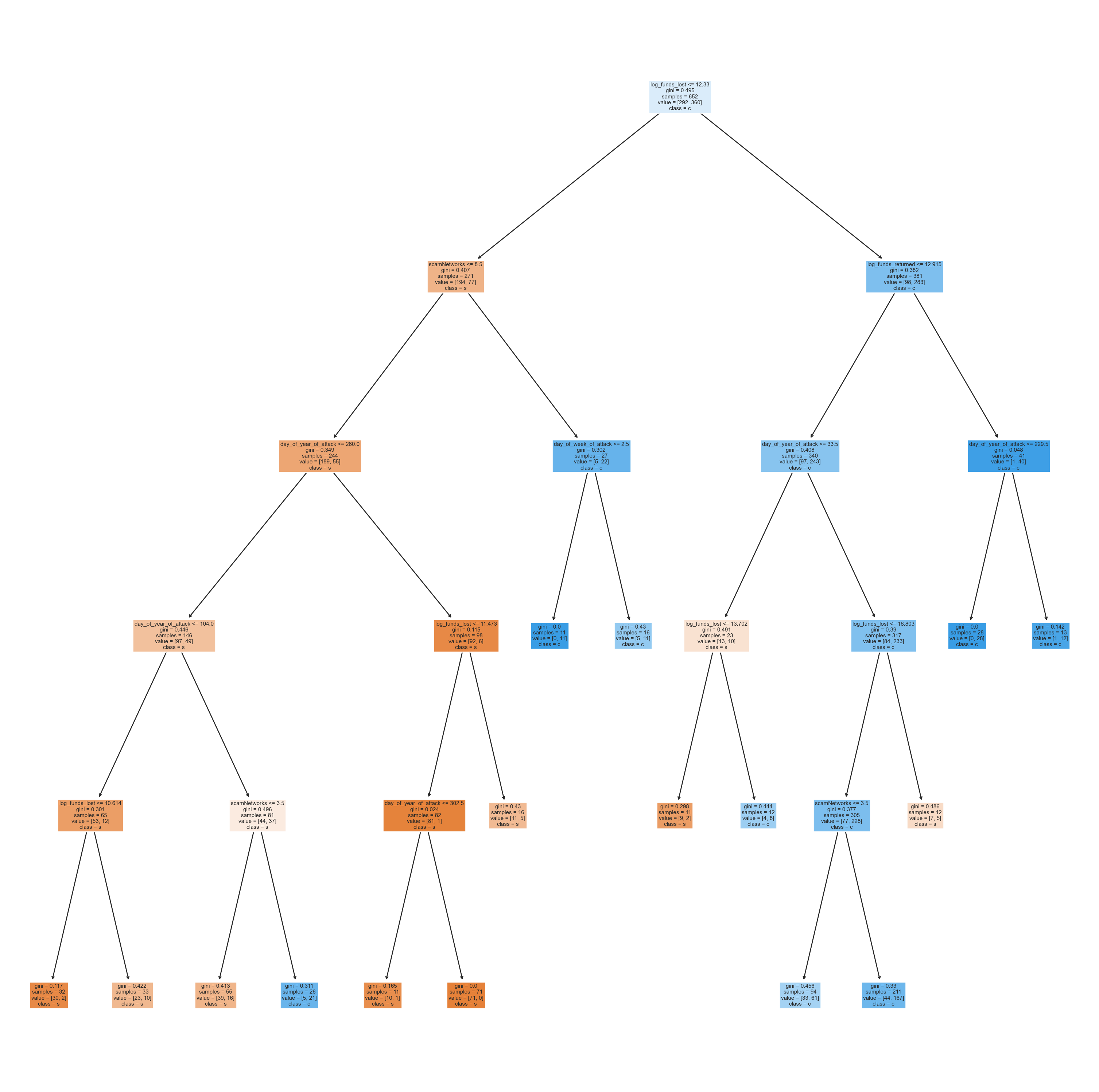
Visualizing the Hyperparameter Tuned Decision Tree
The hyperparameter tuned Tree now outputs a better model that correctly predicts unseen data at 76%, a big boost from 62% as seen in the initial model. The optimum values of the parameters are max_depth = 5 and min_samples_leaf = 10. Therefore, the longer the tree, the more it tends to overfit and we pruned down the extra nodes to gain a lower training accuracy for the benefit of higher test accuracy.
Source Code
---format: html: backgroundcolor: "#63666A" fontcolor: white linkcolor: black code-fold: true code-tools: true df-print: paged highlight-style: vim-darkjupyter: python3---# Binary Classification of Record Data (REKT Database) with Decision TreesThe purpose of this tab is to examine the performance of the Decision Tree Classifier on our cleaned record data gathered from the REKT Database API. and News APIs. If we recall, we conducted multiclass classification on the variable "scam_type" using Naive Bayes in R. For this tab, we shall code in Python and compare the results of the Naive Bayes classifier as well as a baseline random classifier to the results of the Decision Tree Classifier. Like SVM, we shall conduct hyperparameter tuning and try to achieve the lowest training and test errors for our Decision Tree Classifier. ### MethodsBefore we begin modeling our Decision Tree Classifier, we shall test the record data on a random classifier, which is a baseline model, and output its accuracy, precision, and recall values. We shall use sklearn's train-test split function to divide the data into an 80-20 train-test split respectively. Next, we shall employ the Decision Tree Classifier and compare its initial and hyperparameter turned performance with each other and with the random classifier. While performing hyperparameter tuning, we shall use sklearn's GridSearchCV(), like we did for the SVM tab, and change the max_depth, min_samples_leaf, and criterion values. Our goal is to try to achieve the best performing Decision Tree Classifier, which can outperform the Naive Bayes Classifier, which was coded in R. ### ResultsThe cleaned REKT Database has 816 observations after pre-processing. If we recall, the original REKT Database had 3076 observations; however, to treat the heavy class imbalance present in the original data, about 1861 honeypots, 383 rugpulls, and 29 "other" scams were filtered out. Moreover, no key information, in terms of funds lost or source of the attack, was offered about these attacks in the observations that were eliminated. We are left with all those rows where funds lost != 0 and where all projects have some information to offer regarding the extent of the scam, helpful in predicting the scam type. Recalling from the Naive Bayes tab, the initial Naive Bayes Classifier that was tested on the same record data outputted an accuracy of 60% on the test data and the discretized Naive Bayes Classifier outputted an accuracy of 72%. Our expectation is that the Decision Tree should perform better than the Naive Bayes Classifiers because the Decision Tree is a more complex and stronger algorithm than Naive Bayes. Indeed, we are proved correct, as the initial Decision Tree outputted a 100% on all metrics on the training data and a 62% accuracy on the test data. This indicated major overfitting on the training data and, hence, hyperparameter tuning was employed for the Decision Tree to generalize better on unseen data. After performing hyperparameter tuning, the accuracy on the test data was significantly higher at 76%, which means that the Decision Tree did outperform the Naive Bayes Classifier trained on discretized data. Therefore, hyperparameter tuning is an important step in the machine learning process and it opens insights on why and how a particular model performs when its parameters are dialed back and forth.### Loading Libraries and the Cleaned Record Data (REKT Database)```{python}import pandas as pdimport seaborn as sns import matplotlib.pyplot as pltfrom sklearn import treefrom IPython.display import Imageimport numpy as npfrom sklearn.metrics import accuracy_scorefrom sklearn.metrics import precision_scorefrom sklearn.metrics import recall_scorefrom sklearn.metrics import confusion_matrix, ConfusionMatrixDisplay, classification_reportimport warningswarnings.filterwarnings("ignore")``````{python}# LOAD THE DATAFRAMEdf = pd.read_csv("../../data/Clean Data/REKT_Database_Clean_Classification.csv", index_col=[0])``````{python}# Visualize first 5 rowsdf.head(5)``````{python}# PRINT SHAPE print("Data shape is: ", df.shape)```### Exploring the Pre-processed Data using Correlation Heat Maps and PairplotsScam type is the dependent variable, which contains 2 labels, Exit Scam (381 observations) and Exploit (435 observations). The independent variables are a mix of continuous, discrete, and text data. The independent continuous variables are log_funds_lost and log_funds_returned. The independent discrete variables are 3 datetime features, including month_of_attack, day_of_week_of_attack, and day_of_year_of_attack. The only string independent variable is scamNetworks, which denotes the token attached to the project that got scammed.```{python}# RUN THE FOLLOWING CODE TO SHOW THE HEAT-MAP FOR THE CORRELATION MATRIXcorr = df.corr();#print(corr) #COMPUTE CORRELATION OF FEATER MATRIXprint(corr.shape)sns.set_theme(style="white")f, ax = plt.subplots(figsize=(10, 5), dpi=150) # Set up the matplotlib figurecmap = sns.diverging_palette(230, 20, as_cmap=True) # Generate a custom diverging colormap# Draw the heatmap with the mask and correct aspect ratiosns.heatmap(corr, cmap=cmap, vmin=-1, vmax=1, center=0, square=True, linewidths=.5, cbar_kws={"shrink": .5})plt.xticks(rotation=45,fontsize=10)plt.show();# semi colon not needed``````{python}# GENERATING A SEABORN PAIRPLOT sns.pairplot(df,hue="scam_type_grouped", diag_kind='kde')```### Split the dataset into training and testing sets```{python}# MAKE DATA-FRAMES (or numpy arrays) (X,Y) WHERE Y="target" COLUMN and X="everything else"X = df.drop('scam_type_grouped', axis=1)y = df['scam_type_grouped']``````{python}# PARTITION THE DATASET INTO TRAINING AND TEST SETSfrom sklearn.model_selection import train_test_splitx_train, x_test, y_train, y_test = train_test_split(X, y, random_state =1,test_size=0.2)``````{python}# PRINT THE TYPE AND SHAPE OF x_train, x_test, y_train, y_testprint("Shape of x_train is: ", x_train.shape)print("Shape of x_test is: ",x_test.shape)print("Shape of y_train is: ",y_train.shape)print("Shape of y_test is: ",y_test.shape)print("The levels of the dependent variable (Scam Type) are:")print(y.value_counts())```## Baseline Random Classifier```{python}import numpy as npimport randomfrom collections import Counterfrom sklearn.metrics import accuracy_scorefrom sklearn.metrics import precision_recall_fscore_support``````{python}## RANDOM CLASSIFIER def random_classifier(y_data): ypred=[] max_label=np.max(y_data);#print(max_label)for i inrange(0,len(y_data)): ypred.append(int(np.floor((max_label+1)*np.random.uniform(0,1))))print("\n\n-----RANDOM CLASSIFIER-----")print("count of prediction:",Counter(ypred).values()) # counts the elements' frequencyprint("probability of prediction:",np.fromiter(Counter(ypred).values(), dtype=float)/len(y_data)) # counts the elements' frequencyprint("accuracy",accuracy_score(y_data, ypred))print("precision, recall, fscore, support",precision_recall_fscore_support(y_data, ypred))``````{python}from sklearn import preprocessing# label_encoder object knows how to understand word labels.label_encoder = preprocessing.LabelEncoder()# Encode labels in column 'scam_type_grouped' and 'scam_networks'.y_encoded = label_encoder.fit_transform(y)print("\nBINARY CLASS: NON-UNIFORM LOAD (Exit Scam: 381 count, Exploit: 435 count")print("Unique labels and respective counts after one-hot encoding: ")print("0 = Exit Scam and 1 = Exploit")unique, counts = np.unique(y_encoded, return_counts=True)print(np.asarray((unique, counts)).T)random_classifier(y_encoded)```The baseline classifier outputs an overall accuracy of 50% and an f-1 score of 0.0.47630923 for Exit Scam labels and 0.0.4939759 for Exploit labels respectively. The Decision Tree Classifier should perform better than this, let's find out...## Binary Decision Tree Classifier```{python}# One-hot encoding the string column, scam_networks to run the Decision Tree without errorsx_test['scamNetworks'] = label_encoder.fit_transform(x_test['scamNetworks'])x_train['scamNetworks'] = label_encoder.fit_transform(x_train['scamNetworks'])``````{python}#### TRAIN A SKLEARN DECISION TREE MODEL ON x_train,y_train from sklearn import treemodel = tree.DecisionTreeClassifier()model = model.fit(x_train, y_train)``````{python}# USE THE MODEL TO MAKE PREDICTIONS FOR THE TRAINING AND TEST SET from sklearn.metrics import confusion_matrix, ConfusionMatrixDisplayyp_train = model.predict(x_train)yp_test = model.predict(x_test)``````{python}# FUNCTION def confusion_plot(y_data,y_pred) WHICH GENERATES A CONFUSION MATRIX PLOT AND PRINTS THE INFORMATION ABOVE (see link above for example)def confusion_plot(y_data,y_pred): cm = confusion_matrix(y_data, y_pred)print('ACCURACY: {}'.format(accuracy_score(y_data, y_pred)))print('NEGATIVE RECALL (Y=0): {}'.format(recall_score(y_data, y_pred, pos_label='Exit Scam')))print('NEGATIVE PRECISION (Y=0): {}'.format(precision_score(y_data, y_pred, pos_label='Exit Scam')))print('POSITIVE RECALL (Y=1): {}'.format(recall_score(y_data, y_pred, pos_label='Exploit')))print('POSITIVE PRECISION (Y=1): {}'.format(precision_score(y_data, y_pred, pos_label='Exploit')))print(cm)#sns.heatmap(cm, annot=True, fmt='d') ConfusionMatrixDisplay.from_predictions(y_data,y_pred) plt.show()```### Evaluating Initial Decision Tree Performance```{python}# TESTING THE FUNCTION print("------TRAINING------")confusion_plot(y_train,yp_train)print("------TEST------")confusion_plot(y_test,yp_test)```The initial Decision Tree outputted a 100% on all metrics on the training data and a 62% accuracy on the test data. This is a case of major overfitting on the training data! The Decision Tree below outputs a highly complex tree of several child nodes to learn the training data as best as possible. However, this led to it not generalizing well on unseen data, which is why we see a significantly lower accuracy of 62% on the test set. Therefore, we shall employ hyperparameter tuning for the Decision Tree to generalize better on unseen data.### Visualizing the Decision Tree```{python}# FUNCTION "def plot_tree(model,X,Y)" VISUALIZES THE DECISION TREE from dtreeviz.trees import*from sklearn import treedef plot_tree(model, X, Y): plt.figure(figsize=(20, 20)) tree.plot_tree(model, filled=True, feature_names=X.columns, class_names=Y.name) plt.show()plot_tree(model, x_train, y_train)```### Hyper-parameter tuning using GridSearchCV: Evaluating Best Decision Tree Classifier for Test Data PerformanceThe "max_depth" hyper-parameter lets us control the number of layers in our tree.The leaf nodes of the Decision Tree don't split the data any further. Therefore, "min_samples_leaf" hyper-parameter lets us control the classification for examples that end up in that node. We shall iterate over "max_depth" and "min_samples_leaf" as well as change the criterions, including gini and entropy, of judging the best splits to try to find the set of hyper-parameters with the lowest training AND test error.```{python}from sklearn.model_selection import GridSearchCV from sklearn import tree# defining parameter rangeparam_grid = params = {'max_depth': [2, 3, 5, 10, 20],'min_samples_leaf': [5, 10, 20, 50, 100],'criterion': ["gini", "entropy"]}grid = GridSearchCV(tree.DecisionTreeClassifier(), param_grid, refit =True, verbose =-1)grid.fit(x_train, y_train)# print best parameter after tuningprint("The best parameters after tuning are: ", grid.best_params_)# print how our model looks after hyper-parameter tuningprint("The best model after tuning looks like: ",grid.best_estimator_)grid_predictions = grid.predict(x_test)# print classification reportprint(classification_report(y_test, grid_predictions))```### Visualizing the Hyperparameter Tuned Decision Tree```{python}hyperparameter_tuned_best_model = tree.DecisionTreeClassifier(criterion='gini', max_depth=5, min_samples_leaf=10)hyperparameter_tuned_best_model.fit(x_train, y_train)plot_tree(hyperparameter_tuned_best_model, x_train, y_train)```The hyperparameter tuned Tree now outputs a better model that correctly predicts unseen data at 76%, a big boost from 62% as seen in the initial model. The optimum values of the parameters are max_depth = 5 and min_samples_leaf = 10. Therefore, the longer the tree, the more it tends to overfit and we pruned down the extra nodes to gain a lower training accuracy for the benefit of higher test accuracy.