The analysis of the data collected begins from this pivotal section. Every data science project, especially those utilizing Time Series data, starts with Data Visualization because it allows for easy and intuitive interpretation of complex data sets. These visualizations help data scientists identify patterns, trends, and relationships that might otherwise be difficult to discern by looking at the summary statistics the raw data, for example. The visualizations presented below were created using Tableau and the packages ggplot2 and Plotly in the R software.
Visualizing the GTD™
For the purpose of this project, the focus will be on the United States, so the data has been filtered accordingly. An important point to keep in mind is that incidents of terrorism from 1993 are not present in the GTD™ because they were lost by the authors. Hence, few visualizations created in R, using the GTD™, do reflect this aberration, as missing values for the year 1993 were not imputed.
To start, the visualizations below provide a general overview of how the number of terrorist attacks and fatalities have changed over time.
Evolution of Volume of Terrorist Attacks and Fatalaties (1970-2020) in the US
plot_ly(data=gtd_monthly_attacks_deaths, x=~Date) %>%add_trace(type ='scatter', mode ='lines', y=~num_attacks, name="Attacks", line =list(color ='red')) %>%add_trace(type ='scatter', mode ='lines', y=~num_fatal, name="Fatalities", line =list(color ='black')) %>%layout(title="Monthly Count of Terrorist Attacks & Fatalities in the US",yaxis=list(title=("Count")),xaxis=list(title=("Date"))) %>%layout(hovermode ="x")
Code
plot_ly(data=gtd_monthly_attacks_deaths %>%filter(num_fatal<20), x=~Date) %>%add_trace(type ='scatter', mode ='lines', y=~num_attacks, name="Attacks", line =list(color ='red')) %>%add_trace(type ='scatter', mode ='lines', y=~num_fatal, name="Fatalities", line =list(color ='black')) %>%layout(title="Monthly Count of Terrorist Attacks & Fatalities in the US",yaxis=list(title=("Count")),xaxis=list(title=("Date"))) %>%layout(hovermode ="x")
Code
gtd_yearly <- gtd_USA %>%group_by(year(Date)) %>%summarise(num_attacks =n(), nkill=sum(nkill))gtd_yearly_cum_attacks_deaths <- gtd_yearly %>%summarise(cum_attacks=cumsum(num_attacks),cum_deaths =cumsum(nkill)) %>%mutate(Date=gtd_yearly$`year(Date)`)plot_ly(data=gtd_yearly_cum_attacks_deaths, x=~Date) %>%add_trace(type ='scatter', mode ='lines', y=~cum_attacks, name="Cumulative Attacks", line =list(color ='red')) %>%add_trace(type ='scatter', mode ='lines', y=~cum_deaths, name="Cumulative Fatalities", line =list(color ='black')) %>%layout(title="Yearly Cumulative Count of Terrorist Attacks & Fatalities in the US",yaxis=list(title=("Cumulative Count")),xaxis=list(title=("Date"))) %>%layout(hovermode ="x")
The first plot (Number of Monthly Attacks and Fatalities) conveys the significance of the 9/11 Attacks on US history. The big black spike in fatalities, totaling approximately 3000, is representative of the attack and an “outlier” from both series. As a result, in order to depict the trend of both series clearly, it was imperative to filter out the 9/11 Attacks and that is why the second plot was created. A cumulative graph of number of attacks and fatalities is showcased as well that provides further context about the impact of the 9/11 Attacks. Total fatalities were much lower than total number of attakcs from 1970 to 2000, but the toll of the 9/11 Attacks were significant enough to surpass the 2,424 attacks that occurred up until the tragedy.
Moreover, the total number of fatalities between 1970 and 2000 was 492 and the total number of fatalities between 2001 and 2020 was 419, suggesting that attacks apart from 9/11 follow a similar trend in death rate. Lastly, the number of attacks between the years 1976 and 2004 follow a concave shape, implying that the volume of attacks must be diminishing through the years. However, a steep, exponential rise in not only the number of attacks but also the number of fatalities is noticed after 2004!
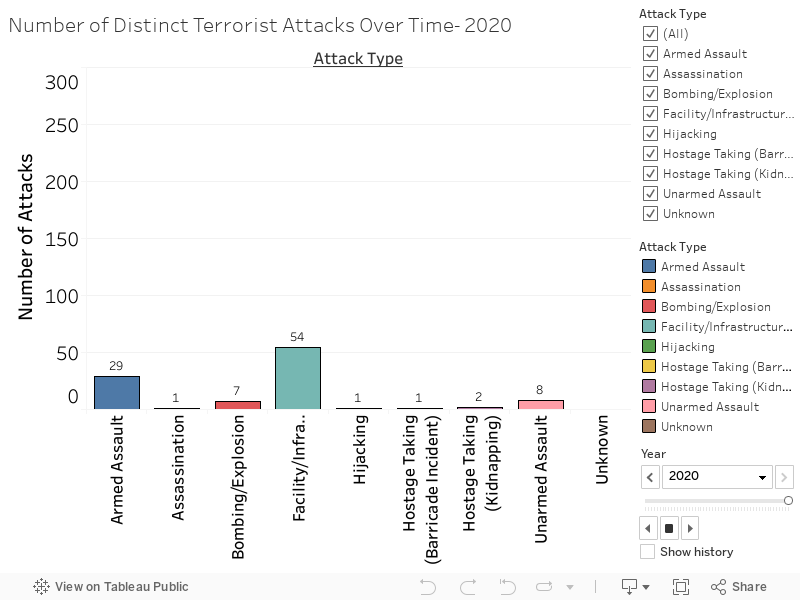
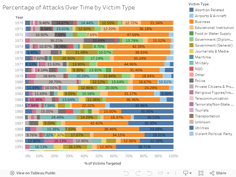
The above bar chart races allow for an animated way to display the number of attacks changing over time by the categorical variables, Attack Type, Victim Type, and Weapon Type. The 1970s and 1980s were dominated by Bombing/Explosion Terrorist Attacks in the US, with Facility/Infrastructure Attacks gaining momentum by the end of the 1980s. Many of these bombings were carried out by leftist extremist groups, such as the Weather Underground and the Black Liberation Army, who were motivated by a variety of political and social causes, including opposition to the Vietnam War, racial injustice, and government oppression (Serrano 2008).
One factor that contributed to the prevalence of domestic bombing attacks during this period was the rise of radical political activism and social unrest. The Vietnam War was a major source of division in American society, and many activists were inspired to use violent tactics in their protests. Additionally, the civil rights movement and the Black Power movement brought attention to issues of racial inequality, and some extremist groups sought to further their agendas through bombings and other violent actions. Another factor was the relative ease with which these groups could obtain explosives and other materials necessary to carry out bombings. Many of the bombs used in these attacks were constructed using readily available materials such as dynamite and pipe bombs, and there were few restrictions on the purchase of these materials at the time (Rosenau, n.d.).
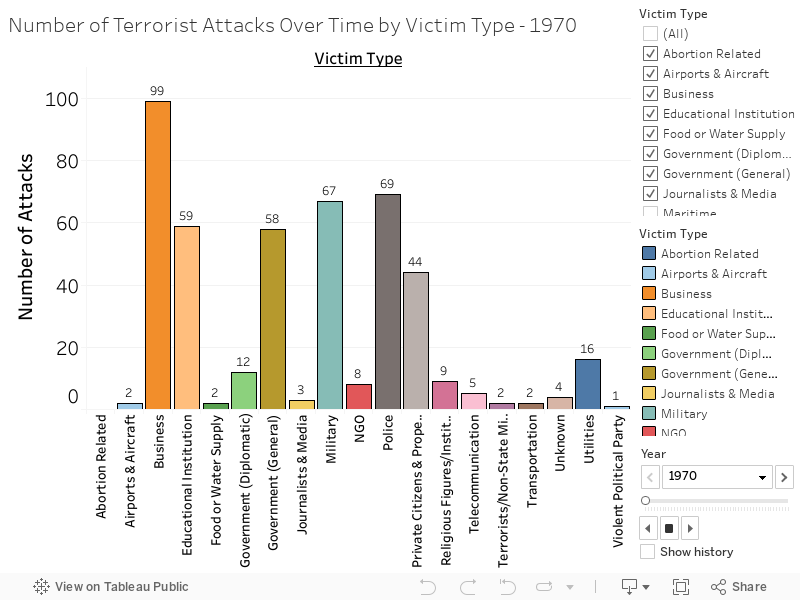
In the 1970s and 1980s, a majority of the victims of these attacks included businesses (corporate offices, restaurants, gas stations, bars, cafés, etc.), the government (government building, government member, former members, or events sponsored by political parties, etc.), and private citizens and property (the public in general or attacks in public areas including markets, commercial streets, busy intersections and pedestrian malls) (“Codebook Methodology Inclusion Criteria and Variables - UMD,” n.d.). Moreover, numerous attacks on abortion clinics were conducted in the 1980s and 1990s by anti-abortion activists. These attacks took various forms, including bombings, arson, and other acts of violence, as well as peaceful protests and acts of civil disobedience. Another factor that contributed to the attacks on abortion clinics was the political and legal context of the time. In 1973, the US Supreme Court issued its landmark decision in Roe v. Wade, which established a constitutional right to abortion. This decision was highly controversial and sparked a wave of political and social activism on both sides of the issue.
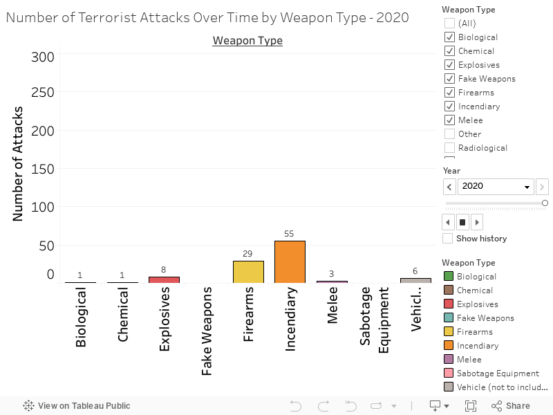
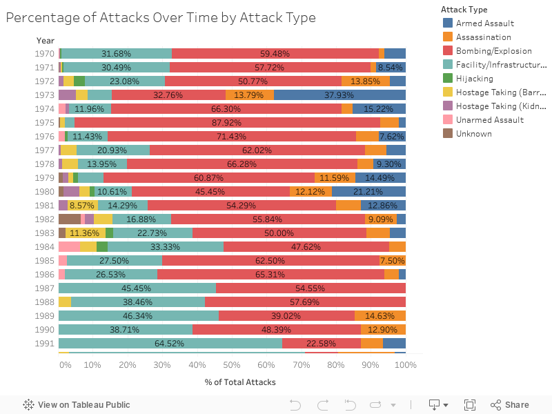
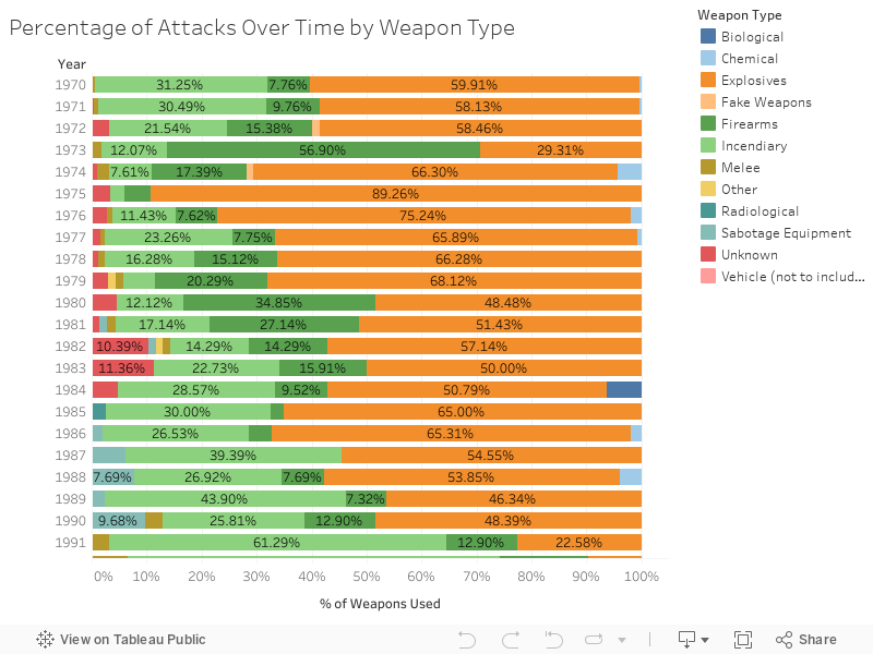
From recent years, the data portrays an increase in attacks against both Religious Figures/Institutions and the police. Therefore, terrorists’ aims and agendas have transformed over time as the underlying narrative of a country’s political climate changes. In a smaller sense, to conduct an attack, the US has also suffered from the evolution of weapons used by terrorists. As aforementioned, the 1970s and 1980s experienced bombings as the majority of attacks and the weapons used during that time support this finding. Explosives and incendiaries made up the majority of weapons used in the 1970s and 1980s, with firearms gaining traction. By the late 90s, less use of explosives is seen and a shift to incendiaries, firearms, chemical, and biological weapons becomes prominent.
94% of attacks against abortion‐related targets were on clinics, while 6% targeted providers or personnel.
78% of attacks against educational targets were on schools, universities, or
other buildings, while 22% targeted teachers or other educational personnel.
73% of attacks against government targets were on government buildings, facilities, or offices, while 27% targeted personnel, public officials, or politicians.
Evolution of Terrorist Attacks: Approach, Victims, and Weapons (Percent of Total)
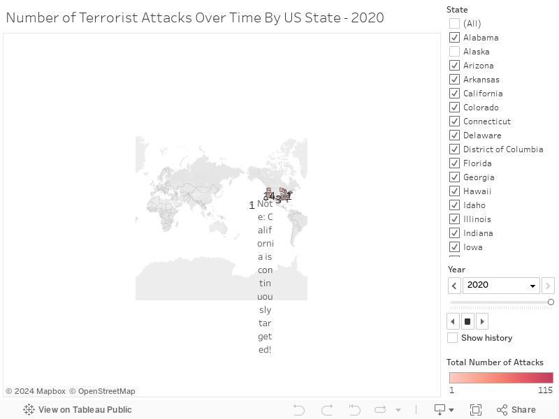
Evolution of Terrorist Attacks By US State (Geospatial)
Visualizing the SIPRI Military Expenditure Database
Code
# new dataframe for total number of attacks 1970-2020sipri_usa <- sipri_gdp %>%filter(Country=="United States of America")# transpose to make columns into rowssipri_usa <-as.data.frame(t(sipri_usa))sipri_usa <-as.numeric(sipri_usa[-1,]) # delete first row sipri_usa <-round(sipri_usa*100, 4)# convert to time series objectsipri_usa_ts <-ts(sipri_usa, start =c(1949), frequency =1)g <-autoplot(sipri_usa_ts, main="Yearly US Military Expenditure as % of GDP",ylab ="Military Expenditure as % of GDP",xlab ="Date") +theme_minimal()ggplotly(g) %>%layout(hovermode ="x")
Visualizing Department of Homeland Security’s Non-Immigrant Admissions Data
Code
dhs <- dhs %>%filter(Year>=2002)fig <-plot_ly(dhs, x =~Year, y =~`Temporaryvisitorsforpleasure(B2)`,name ='B2 Tourist Visa Holders', type ='scatter', mode ='lines')fig <- fig %>%add_trace(y =~`Temporaryvisitorsforbusiness(B1)`, name ='B1 Business Visa Holders', type ='scatter', mode ='lines')fig <- fig %>%add_trace(y =~`Academicstudents(F1)`, name ='F1 Student Visa Holders', type ='scatter', mode ='lines')fig <- fig %>%layout(title ='Select Non-Immigrant Admissions 2002-2021',yaxis=list(title ='Number of Admissions (in millions)'))fig
---title: "Data Visualization"format: html: page-layout: full code-fold: show code-copy: true code-tools: true code-overflow: wrapbibliography: bibliography.bib---## SummaryThe analysis of the data collected begins from this pivotal section. Every data science project, especially those utilizing Time Series data, starts with Data Visualization because it allows for easy and intuitive interpretation of complex data sets. These visualizations help data scientists identify patterns, trends, and relationships that might otherwise be difficult to discern by looking at the summary statistics the raw data, for example. The visualizations presented below were created using *Tableau* and the packages `ggplot2` and `Plotly` in the *R software*. ## Visualizing the GTD™For the purpose of this project, the focus will be on the United States, so the data has been filtered accordingly. An important point to keep in mind is that incidents of terrorism from 1993 are not present in the GTD™ because they were lost by the authors. Hence, few visualizations created in R, using the GTD™, do reflect this aberration, as missing values for the year 1993 were not imputed. To start, the visualizations below provide a general overview of how the number of terrorist attacks and fatalities have changed over time. ```{r,include=FALSE, message=FALSE, warning=FALSE}library(flipbookr)library(tidyverse)library(ggplot2)library(forecast)library(astsa) library(xts)library(tseries)library(fpp2)library(fma)library(lubridate)library(tidyverse)library(TSstudio)library(quantmod)library(tidyquant)library(plotly)library(ggplot2)library(padr)``````{r load,include=FALSE, message=FALSE, warning=FALSE}gtd <- readxl::read_xlsx("../Data/gtd.xlsx")sipri_gdp <- readxl::read_xlsx("../Data/SIPRI_GDP.xlsx")sipri_region <- readxl::read_xlsx("../Data/SIPRI_Region.xlsx")dhs <- readxl::read_xls("../Data/DHS_98_21.xls")``````{r createdate,include=FALSE, message=FALSE, warning=FALSE}# if the exact day/month of the event is unknown, this is recorded as “0”gtd$Date <-as.Date(with(gtd,paste(iyear,imonth,iday,sep="-")),"%Y-%m-%d")# results in 891 NAs total, 33 of which correspond to country_txt==USA``````{r filterUS,include=FALSE, message=FALSE, warning=FALSE}# Filter country_txt==USAgtd_USA <- gtd %>%filter(country_txt=="United States")# drop 33 observations from a total of 3121 observations (if taking for '70)gtd_USA <- gtd_USA[complete.cases(gtd_USA$Date),]# impute missing values for nkill (Total Number of Fatalities: victims and attackers) as 0gtd_USA$nkill[is.na(gtd_USA$nkill)] <-0# select desired columns for analysisgtd_USA <- gtd_USA %>%select(Date, provstate, city, attacktype1_txt, targtype1_txt, gname, nkill, nkillus, weaptype1_txt)``````{r monthlyattdeath,include=FALSE, message=FALSE, warning=FALSE}# new dataframe for monthly number of attacks 1970-2020gtd_monthly_attacks_deaths <- gtd_USA %>%group_by(year(Date), month(Date)) %>%summarise(num_attacks =n(), nkill=sum(nkill))colnames(gtd_monthly_attacks_deaths)[1] ="Year"colnames(gtd_monthly_attacks_deaths)[2] ="Month"colnames(gtd_monthly_attacks_deaths)[4] ="num_fatal"gtd_monthly_attacks_deaths$Date <-as.Date(paste0(gtd_monthly_attacks_deaths$Year, "-", gtd_monthly_attacks_deaths$Month, "-01"), "%Y-%m-%d")#as.Date(with(gtd_monthly_attacks_deaths,paste(Year,Month,sep="-")),"%Y-%m")# Fill missing dates (0 attacks for those dates)gtd_monthly_attacks_deaths <- gtd_monthly_attacks_deaths %>%complete(Date =seq.Date(min(Date), max(Date), by="month")) gtd_monthly_attacks_deaths <-pad(gtd_monthly_attacks_deaths) %>%replace(is.na(.), 0)```### Evolution of Volume of Terrorist Attacks and Fatalaties (1970-2020) in the US::: panel-tabset#### Number of Monthly Attacks and Fatalities ```{r plot1, message=FALSE, warning=FALSE}plot_ly(data=gtd_monthly_attacks_deaths, x=~Date) %>%add_trace(type ='scatter', mode ='lines', y=~num_attacks, name="Attacks", line =list(color ='red')) %>%add_trace(type ='scatter', mode ='lines', y=~num_fatal, name="Fatalities", line =list(color ='black')) %>%layout(title="Monthly Count of Terrorist Attacks & Fatalities in the US",yaxis=list(title=("Count")),xaxis=list(title=("Date"))) %>%layout(hovermode ="x")```#### Number of Monthly Attacks and Fatalities (adjusted for 9/11)```{r plot2, message=FALSE, warning=FALSE}plot_ly(data=gtd_monthly_attacks_deaths %>%filter(num_fatal<20), x=~Date) %>%add_trace(type ='scatter', mode ='lines', y=~num_attacks, name="Attacks", line =list(color ='red')) %>%add_trace(type ='scatter', mode ='lines', y=~num_fatal, name="Fatalities", line =list(color ='black')) %>%layout(title="Monthly Count of Terrorist Attacks & Fatalities in the US",yaxis=list(title=("Count")),xaxis=list(title=("Date"))) %>%layout(hovermode ="x")```#### Cumulative Count of Terrorist Attacks & Fatalities ```{r yearlycumattdeath, message=FALSE, warning=FALSE}gtd_yearly <- gtd_USA %>%group_by(year(Date)) %>%summarise(num_attacks =n(), nkill=sum(nkill))gtd_yearly_cum_attacks_deaths <- gtd_yearly %>%summarise(cum_attacks=cumsum(num_attacks),cum_deaths =cumsum(nkill)) %>%mutate(Date=gtd_yearly$`year(Date)`)plot_ly(data=gtd_yearly_cum_attacks_deaths, x=~Date) %>%add_trace(type ='scatter', mode ='lines', y=~cum_attacks, name="Cumulative Attacks", line =list(color ='red')) %>%add_trace(type ='scatter', mode ='lines', y=~cum_deaths, name="Cumulative Fatalities", line =list(color ='black')) %>%layout(title="Yearly Cumulative Count of Terrorist Attacks & Fatalities in the US",yaxis=list(title=("Cumulative Count")),xaxis=list(title=("Date"))) %>%layout(hovermode ="x")```:::The first plot (Number of Monthly Attacks and Fatalities) conveys the significance of the 9/11 Attacks on US history. The big black spike in fatalities, totaling approximately 3000, is representative of the attack and an "outlier" from both series. As a result, in order to depict the trend of both series clearly, it was imperative to filter out the 9/11 Attacks and that is why the second plot was created. A cumulative graph of number of attacks and fatalities is showcased as well that provides further context about the impact of the 9/11 Attacks. Total fatalities were much lower than total number of attakcs from 1970 to 2000, but the toll of the 9/11 Attacks were significant enough to surpass the 2,424 attacks that occurred up until the tragedy.Moreover, the total number of fatalities between 1970 and 2000 was 492 and the total number of fatalities between 2001 and 2020 was 419, suggesting that attacks apart from 9/11 follow a similar trend in death rate. Lastly, the number of attacks between the years 1976 and 2004 follow a concave shape, implying that the volume of attacks must be diminishing through the years. However, a steep, exponential rise in not only the number of attacks but also the number of fatalities is noticed after 2004!Here are a few facts [@GTDfacts] attacks in the US between 1970 and 2013: - Approximately 85% of all deaths from terrorist attacks during this period occurred in the coordinated attacks on September 11, 2001. - Nearly 80% of all terrorist attacks involved no casualties (fatalities or injuries). - More than half of terrorist attacks took place during the 1970s. Between 2000 and 2013, there were fewer than 20 attacks per year on average.```{r groupedbarcsv, include=FALSE, message=FALSE, warning=FALSE}grouped_year_attacks <- gtd_USA %>%group_by(year(Date), attacktype1_txt) %>%summarize(attacks =n())colnames(grouped_year_attacks)[1] ="Year"colnames(grouped_year_attacks)[2] ="Attack_Type"write.csv(grouped_year_attacks, "../Data/Grouped_Year_Attacks.csv")grouped_year_targets <- gtd_USA %>%group_by(year(Date), targtype1_txt) %>%summarize(targets =n())colnames(grouped_year_targets)[1] ="Year"colnames(grouped_year_targets)[2] ="Target_Type"write.csv(grouped_year_targets, "../Data/Grouped_Year_Targets.csv")grouped_year_weapons <- gtd_USA %>%group_by(year(Date), weaptype1_txt) %>%summarize(weapons =n())colnames(grouped_year_weapons)[1] ="Year"colnames(grouped_year_weapons)[2] ="Weapon_Type"write.csv(grouped_year_weapons, "../Data/Grouped_Year_Weapons.csv")grouped_year_states <- gtd_USA %>%group_by(year(Date), provstate) %>%summarize(attacks =n())colnames(grouped_year_states)[1] ="Year"colnames(grouped_year_states)[2] ="State"write.csv(grouped_year_states, "../Data/Grouped_Year_States.csv")```### Evolution of Terrorist Attacks: Approach, Victims, and Weapons (Raw Counts)::: panel-tabset#### Number of Distinct Attacks Over Time<divclass='tableauPlaceholder'id='viz1676603864684'style='position: relative'><noscript><ahref='#'><imgalt='Number of Distinct Terrorist Attacks Over Time- 2020 'src='https://public.tableau.com/static/images/Ti/TimeSeriesProject-NumberofDistinctTerroristAttacksOverTime1970-2020/Sheet3/1_rss.png'style='border: none'/></a></noscript><objectclass='tableauViz'style='display:none;'><paramname='host_url'value='https%3A%2F%2Fpublic.tableau.com%2F'/><paramname='embed_code_version'value='3'/><paramname='site_root'value=''/><paramname='name'value='TimeSeriesProject-NumberofDistinctTerroristAttacksOverTime1970-2020/Sheet3'/><paramname='tabs'value='no'/><paramname='toolbar'value='yes'/><paramname='static_image'value='https://public.tableau.com/static/images/Ti/TimeSeriesProject-NumberofDistinctTerroristAttacksOverTime1970-2020/Sheet3/1.png'/><paramname='animate_transition'value='yes'/><paramname='display_static_image'value='yes'/><paramname='display_spinner'value='yes'/><paramname='display_overlay'value='yes'/><paramname='display_count'value='yes'/><paramname='language'value='en-US'/><paramname='filter'value='publish=yes'/></object></div>```{js, tableau1, echo=FALSE}var divElement =document.getElementById('viz1676603864684');var vizElement = divElement.getElementsByTagName('object')[0]; vizElement.style.width='100%';vizElement.style.height=(divElement.offsetWidth*0.75)+'px';var scriptElement =document.createElement('script'); scriptElement.src='https://public.tableau.com/javascripts/api/viz_v1.js'; vizElement.parentNode.insertBefore(scriptElement, vizElement);```#### Trends in Attacks Over Time by Victim Type {.active}<div class='tableauPlaceholder' id='viz1676603919579' style='position: relative'><noscript><a href='#'><img alt='Number of Terrorist Attacks Over Time by Victim Type - 1970 ' src='https://public.tableau.com/static/images/Ti/TimeSeriesProject-NumberofTerroristAttacksOverTimebyVictimType1970-2020/Sheet3/1_rss.png' style='border: none' /></a></noscript><object class='tableauViz' style='display:none;'><param name='host_url' value='https%3A%2F%2Fpublic.tableau.com%2F' /> <param name='embed_code_version' value='3' /> <param name='site_root' value='' /><param name='name' value='TimeSeriesProject-NumberofTerroristAttacksOverTimebyVictimType1970-2020/Sheet3' /><param name='tabs' value='no' /><param name='toolbar' value='yes' /><param name='static_image' value='https://public.tableau.com/static/images/Ti/TimeSeriesProject-NumberofTerroristAttacksOverTimebyVictimType1970-2020/Sheet3/1.png' /> <param name='animate_transition' value='yes' /><param name='display_static_image' value='yes' /><param name='display_spinner' value='yes' /><param name='display_overlay' value='yes' /><param name='display_count' value='yes' /><param name='language' value='en-US' /><param name='filter' value='publish=yes' /></object></div> ```{js, tableau2, echo=FALSE}var divElement =document.getElementById('viz1676603919579');var vizElement = divElement.getElementsByTagName('object')[0]; vizElement.style.width='100%';vizElement.style.height=(divElement.offsetWidth*0.75)+'px';var scriptElement =document.createElement('script'); scriptElement.src='https://public.tableau.com/javascripts/api/viz_v1.js'; vizElement.parentNode.insertBefore(scriptElement, vizElement);```#### Trends in Attacks Over Time by Weapon Type {.active}<div class='tableauPlaceholder' id='viz1676664015615' style='position: relative'><noscript><a href='#'><img alt='Number of Terrorist Attacks Over Time by Weapon Type - 2020 ' src='https://public.tableau.com/static/images/Ti/TimeSeriesProject-NumberofTerroristAttacksOverTimeByWeaponType1970-2020/Sheet3/1_rss.png' style='border: none' /></a></noscript><object class='tableauViz' style='display:none;'><param name='host_url' value='https%3A%2F%2Fpublic.tableau.com%2F' /> <param name='embed_code_version' value='3' /> <param name='site_root' value='' /><param name='name' value='TimeSeriesProject-NumberofTerroristAttacksOverTimeByWeaponType1970-2020/Sheet3' /><param name='tabs' value='no' /><param name='toolbar' value='yes' /><param name='static_image' value='https://public.tableau.com/static/images/Ti/TimeSeriesProject-NumberofTerroristAttacksOverTimeByWeaponType1970-2020/Sheet3/1.png' /> <param name='animate_transition' value='yes' /><param name='display_static_image' value='yes' /><param name='display_spinner' value='yes' /><param name='display_overlay' value='yes' /><param name='display_count' value='yes' /><param name='language' value='en-US' /><param name='filter' value='publish=yes' /></object></div> ```{js, tableau3, echo=FALSE}var divElement =document.getElementById('viz1676664015615');var vizElement = divElement.getElementsByTagName('object')[0]; vizElement.style.width='100%';vizElement.style.height=(divElement.offsetWidth*0.75)+'px';var scriptElement =document.createElement('script'); scriptElement.src='https://public.tableau.com/javascripts/api/viz_v1.js'; vizElement.parentNode.insertBefore(scriptElement, vizElement);```:::The above bar chart races allow for an animated way to display the number of attacks changing over time by the categorical variables, Attack Type, Victim Type, and Weapon Type. The 1970s and 1980s were dominated by Bombing/Explosion Terrorist Attacks in the US, with Facility/Infrastructure Attacks gaining momentum by the end of the 1980s. Many of these bombings were carried out by leftist extremist groups, such as the Weather Underground and the Black Liberation Army, who were motivated by a variety of political and social causes, including opposition to the Vietnam War, racial injustice, and government oppression [@serrano_2008].One factor that contributed to the prevalence of domestic bombing attacks during this period was the rise of radical political activism and social unrest. The Vietnam War was a major source of division in American society, and many activists were inspired to use violent tactics in their protests. Additionally, the civil rights movement and the Black Power movement brought attention to issues of racial inequality, and some extremist groups sought to further their agendas through bombings and other violent actions. Another factor was the relative ease with which these groups could obtain explosives and other materials necessary to carry out bombings. Many of the bombs used in these attacks were constructed using readily available materials such as dynamite and pipe bombs, and there were few restrictions on the purchase of these materials at the time [@rosenau].In the 1970s and 1980s, a majority of the victims of these attacks included businesses (corporate offices, restaurants, gas stations, bars, cafés, etc.), the government (government building, government member, former members, or events sponsored by political parties, etc.), and private citizens and property (the public in general or attacks in public areas including markets, commercial streets, busy intersections and pedestrian malls) [@GTD]. Moreover, numerous attacks on abortion clinics were conducted in the 1980s and 1990s by anti-abortion activists. These attacks took various forms, including bombings, arson, and other acts of violence, as well as peaceful protests and acts of civil disobedience. Another factor that contributed to the attacks on abortion clinics was the political and legal context of the time. In 1973, the US Supreme Court issued its landmark decision in Roe v. Wade, which established a constitutional right to abortion. This decision was highly controversial and sparked a wave of political and social activism on both sides of the issue.From recent years, the data portrays an increase in attacks against both Religious Figures/Institutions and the police. Therefore, terrorists' aims and agendas have transformed over time as the underlying narrative of a country's political climate changes. In a smaller sense, to conduct an attack, the US has also suffered from the evolution of weapons used by terrorists. As aforementioned, the 1970s and 1980s experienced bombings as the majority of attacks and the weapons used during that time support this finding. Explosives and incendiaries made up the majority of weapons used in the 1970s and 1980s, with firearms gaining traction. By the late 90s, less use of explosives is seen and a shift to incendiaries, firearms, chemical, and biological weapons becomes prominent. Here are some more facts [@GTDfacts] related to the bar chart races:- 94% of attacks against abortion‐related targets were on clinics, while 6% targeted providers or personnel. - 78% of attacks against educational targets were on schools, universities, or other buildings, while 22% targeted teachers or other educational personnel. - 73% of attacks against government targets were on government buildings, facilities, or offices, while 27% targeted personnel, public officials, or politicians. ### Evolution of Terrorist Attacks: Approach, Victims, and Weapons (Percent of Total)::: panel-tabset#### Percentage of Distinct Attacks Over Time<div class='tableauPlaceholder' id='viz1676506739847' style='position: relative'><noscript><a href='#'><img alt='Percentage of Attacks Over Time by Attack Type ' src='https://public.tableau.com/static/images/Ti/TimeSeriesProject-PercentageofAttacksOverTimebyAttackType/Sheet2/1_rss.png' style='border: none' /></a></noscript><object class='tableauViz' style='display:none;'><param name='host_url' value='https%3A%2F%2Fpublic.tableau.com%2F' /> <param name='embed_code_version' value='3' /> <param name='site_root' value='' /><param name='name' value='TimeSeriesProject-PercentageofAttacksOverTimebyAttackType/Sheet2' /><param name='tabs' value='no' /><param name='toolbar' value='yes' /><param name='static_image' value='https://public.tableau.com/static/images/Ti/TimeSeriesProject-PercentageofAttacksOverTimebyAttackType/Sheet2/1.png' /> <param name='animate_transition' value='yes' /><param name='display_static_image' value='yes' /><param name='display_spinner' value='yes' /><param name='display_overlay' value='yes' /><param name='display_count' value='yes' /><param name='language' value='en-US' /><param name='filter' value='publish=yes' /></object></div> ```{js, tableau4, echo=FALSE}var divElement =document.getElementById('viz1676506739847');var vizElement = divElement.getElementsByTagName('object')[0]; vizElement.style.width='100%';vizElement.style.height=(divElement.offsetWidth*0.75)+'px';var scriptElement =document.createElement('script'); scriptElement.src='https://public.tableau.com/javascripts/api/viz_v1.js'; vizElement.parentNode.insertBefore(scriptElement, vizElement);```#### Percentage of Attacks Over Time by Victim Type {.active}<div class='tableauPlaceholder' id='viz1676506914339' style='position: relative'><noscript><a href='#'><img alt='Percentage of Attacks Over Time by Victim Type ' src='https://public.tableau.com/static/images/Ti/TimeSeriesProject-PercentageofAttacksOverTimebyVictimType/Sheet2/1_rss.png' style='border: none' /></a></noscript><object class='tableauViz' style='display:none;'><param name='host_url' value='https%3A%2F%2Fpublic.tableau.com%2F' /> <param name='embed_code_version' value='3' /> <param name='site_root' value='' /><param name='name' value='TimeSeriesProject-PercentageofAttacksOverTimebyVictimType/Sheet2' /><param name='tabs' value='no' /><param name='toolbar' value='yes' /><param name='static_image' value='https://public.tableau.com/static/images/Ti/TimeSeriesProject-PercentageofAttacksOverTimebyVictimType/Sheet2/1.png' /> <param name='animate_transition' value='yes' /><param name='display_static_image' value='yes' /><param name='display_spinner' value='yes' /><param name='display_overlay' value='yes' /><param name='display_count' value='yes' /><param name='language' value='en-US' /><param name='filter' value='publish=yes' /></object></div> ```{js, tableau5, echo=FALSE}var divElement =document.getElementById('viz1676506914339');var vizElement = divElement.getElementsByTagName('object')[0]; vizElement.style.width='100%';vizElement.style.height=(divElement.offsetWidth*0.75)+'px';var scriptElement =document.createElement('script'); scriptElement.src='https://public.tableau.com/javascripts/api/viz_v1.js'; vizElement.parentNode.insertBefore(scriptElement, vizElement);```#### Percentage of Attacks Over Time by Weapon Type {.active}<div class='tableauPlaceholder' id='viz1676505947867' style='position: relative'><noscript><a href='#'><img alt='Percentage of Attacks Over Time by Weapon Type ' src='https://public.tableau.com/static/images/Ti/Time-Series-Project-WeaponTypePercent/Sheet2/1_rss.png' style='border: none' /></a></noscript><object class='tableauViz' style='display:none;'><param name='host_url' value='https%3A%2F%2Fpublic.tableau.com%2F' /> <param name='embed_code_version' value='3' /> <param name='site_root' value='' /><param name='name' value='Time-Series-Project-WeaponTypePercent/Sheet2' /><param name='tabs' value='no' /><param name='toolbar' value='yes' /><param name='static_image' value='https://public.tableau.com/static/images/Ti/Time-Series-Project-WeaponTypePercent/Sheet2/1.png' /> <param name='animate_transition' value='yes' /><param name='display_static_image' value='yes' /><param name='display_spinner' value='yes' /><param name='display_overlay' value='yes' /><param name='display_count' value='yes' /><param name='language' value='en-US' /><param name='filter' value='publish=yes' /></object></div> ```{js, tableau6, echo=FALSE}var divElement =document.getElementById('viz1676505947867');var vizElement = divElement.getElementsByTagName('object')[0]; vizElement.style.width='100%';vizElement.style.height=(divElement.offsetWidth*0.75)+'px';var scriptElement =document.createElement('script'); scriptElement.src='https://public.tableau.com/javascripts/api/viz_v1.js'; vizElement.parentNode.insertBefore(scriptElement, vizElement);```:::### Evolution of Terrorist Attacks By US State (Geospatial)<div class='tableauPlaceholder' id='viz1676609472785' style='position: relative'><noscript><a href='#'><img alt='Number of Terrorist Attacks Over Time By US State - 2020 ' src='https://public.tableau.com/static/images/4D/4D5BQMGF4/1_rss.png' style='border: none' /></a></noscript><object class='tableauViz' style='display:none;'><param name='host_url' value='https%3A%2F%2Fpublic.tableau.com%2F' /> <param name='embed_code_version' value='3' /> <param name='path' value='shared/4D5BQMGF4' /> <param name='toolbar' value='yes' /><param name='static_image' value='https://public.tableau.com/static/images/4D/4D5BQMGF4/1.png' /> <param name='animate_transition' value='yes' /><param name='display_static_image' value='yes' /><param name='display_spinner' value='yes' /><param name='display_overlay' value='yes' /><param name='display_count' value='yes' /><param name='language' value='en-US' /><param name='filter' value='publish=yes' /></object></div> ```{js, tableau7, echo=FALSE}var divElement =document.getElementById('viz1676609472785');var vizElement = divElement.getElementsByTagName('object')[0]; vizElement.style.width='100%';vizElement.style.height=(divElement.offsetWidth*0.75)+'px';var scriptElement =document.createElement('script'); scriptElement.src='https://public.tableau.com/javascripts/api/viz_v1.js'; vizElement.parentNode.insertBefore(scriptElement, vizElement);```## Visualizing the SIPRI Military Expenditure Database```{r sipri,message=FALSE, warning=FALSE}# new dataframe for total number of attacks 1970-2020sipri_usa <- sipri_gdp %>%filter(Country=="United States of America")# transpose to make columns into rowssipri_usa <-as.data.frame(t(sipri_usa))sipri_usa <-as.numeric(sipri_usa[-1,]) # delete first row sipri_usa <-round(sipri_usa*100,4)# convert to time series objectsipri_usa_ts <-ts(sipri_usa, start =c(1949), frequency =1)g <-autoplot(sipri_usa_ts, main="Yearly US Military Expenditure as % of GDP", ylab ="Military Expenditure as % of GDP", xlab ="Date") +theme_minimal()ggplotly(g) %>%layout(hovermode ="x")```## Visualizing Department of Homeland Security's Non-Immigrant Admissions Data```{r dhs, message=FALSE, warning=FALSE}dhs <- dhs %>%filter(Year>=2002)fig <-plot_ly(dhs, x =~Year, y =~`Temporaryvisitorsforpleasure(B2)`,name ='B2 Tourist Visa Holders', type ='scatter', mode ='lines')fig <- fig %>%add_trace(y =~`Temporaryvisitorsforbusiness(B1)`, name ='B1 Business Visa Holders', type ='scatter', mode ='lines')fig <- fig %>%add_trace(y =~`Academicstudents(F1)`, name ='F1 Student Visa Holders', type ='scatter', mode ='lines')fig <- fig %>%layout(title ='Select Non-Immigrant Admissions 2002-2021', yaxis=list(title ='Number of Admissions (in millions)'))fig```## Section Code**Code for this section can be found [here](https://github.com/TegveerG/Time-Series-Project/blob/main/Time%20Series%20Analysis/Data-Visualization.qmd)**