Financial Time Series Models

Summary

In the previous parts of this study, the focus was on utilizing models that capture the conditional mean structure of time series data. However, for financial time series, the conditional variance structure can be modeled using ARCH and GARCH models. Typically, periods of high volatility, a statistical measure of the dispersion of returns, for a given security or market index are followed by higher conditional variance compared to stable periods. This is known as volatility clustering. ARCH/GARCH models are designed to capture the time-varying variance of returns or to predict the conditional variance of a time series, which help us forecast the volatility of future returns.

Autoregressive Conditional Heteroscedasticity (ARCH) refers to a model that applies an autoregressive component to the variance of a univariate time series. Although an ARCH model could possibly be used to describe a gradually increasing variance over time, most often it is used in situations in which there may be short periods of increased variation. Specifically, the ARCH(p) model models the returns as:

\(r_t = log(x_t) − log(x_{t−1})\)

\(r_t = \sigma_t \epsilon_t\)

\(\sigma^2_t = Var(r_t|r_{t-1}) = a_0 + a_1r_{t-1}^2 + ... + a_pr_{t-p}^2\), where \(\epsilon_t\) is standard Gaussian white noise.

Generalized Autoregressive Conditional Heteroskedasticity (GARCH) is an extension of the ARCH model that incorporates a moving average component together with the autoregressive component. The introduction of a moving average component allows the model to both model the conditional change in variance over time as well as changes in the time-dependent variance. Just like ARCH(p) is AR(p) applied to the variance of a time series, GARCH(p, q) is an ARMA(p,q) model applied to the variance of a time series. Specifically, the GARCH(p,q) model models the returns as:

\(r_t = \sigma_t \epsilon_t\)

\(\begin{equation}\sigma_t^2 = a_0 + \sum_{j=1}^{p} \alpha_j r_{t-j}^2 + \sum_{j=1}^{q} \beta_j \sigma_{t-j}^2\end{equation}\), where \(\epsilon_t\) is standard Gaussian white noise, \(\alpha_j\) and \(\beta_j\) are the coefficients for the lagged squared residuals and lagged conditional variances, respectively. The model is called a GARCH(p,q) model if it includes \(p\) lags of the squared residuals and \(q\) lags of the conditional variances.

In financial time series analysis, it is common practice to fit an ARMA model to the data to capture the conditional mean structure, followed by the application of an ARCH or GARCH model to model the conditional variance. The upcoming section will apply this approach to model 3 financial time series, including Lockheed Martin, Raytheon Technologies, and Dow Jones U.S. Travel & Tourism Index, using a combination of ARMA and GARCH models.

Visualizing Financial Time Series

Lockheed Martin (LMT)

Code

lmt$SMA_50 <- as.numeric(SMA(Cl(lmt),n=50))
lmt$SMA_200 <- as.numeric(SMA(Cl(lmt),n=200))

fig <- lmt %>% plot_ly(x = ~Date, type="candlestick",
          open = ~LMT.Open, close = ~LMT.Close,
          high = ~LMT.High, low = ~LMT.Low, name = "Candlestick") %>% 
  add_trace(type = 'scatter', mode = 'lines', y=~SMA_50, 
            name="SMA_50", line = list(color = 'blue')) %>% 
  add_trace(type = 'scatter', mode = 'lines', y=~SMA_200, 
            name="SMA_200",line = list(color = 'orange')) 
fig <- fig %>%
  layout(title = "LMT Candlestick Chart with 50 And 200 Day Simple Moving-Average") %>% 
  layout(hovermode = "x") %>%
  layout(paper_bgcolor = "black",
         plot_bgcolor = "black",
         font = list(color = "white"),
         yaxis = list(linecolor = "#6b6b6b",
                      zerolinecolor = "#6b6b6b",
                      gridcolor= "#444444"),
         xaxis = list(linecolor = "#6b6b6b",
                      zerolinecolor = "#6b6b6b",
                      gridcolor= "#444444"))

fig

Raytheon Technologies (RTX)

Code

rtx$SMA_50 <- as.numeric(SMA(Cl(rtx),n=50))
rtx$SMA_200 <- as.numeric(SMA(Cl(rtx),n=200))

fig <- rtx %>% plot_ly(x = ~Date, type="candlestick",
          open = ~RTX.Open, close = ~RTX.Close,
          high = ~RTX.High, low = ~RTX.Low, name = "Candlestick") %>% 
  add_trace(type = 'scatter', mode = 'lines', y=~SMA_50, 
            name="SMA_50", line = list(color = 'blue')) %>% 
  add_trace(type = 'scatter', mode = 'lines', y=~SMA_200, 
            name="SMA_200",line = list(color = 'orange')) 
fig <- fig %>%
  layout(title = "RTX Candlestick Chart with 50 And 200 Day Simple Moving-Average") %>% 
  layout(hovermode = "x") %>%
  layout(paper_bgcolor = "black",
         plot_bgcolor = "black",
         font = list(color = "white"),
         yaxis = list(linecolor = "#6b6b6b",
                      zerolinecolor = "#6b6b6b",
                      gridcolor= "#444444"),
         xaxis = list(linecolor = "#6b6b6b",
                      zerolinecolor = "#6b6b6b",
                      gridcolor= "#444444"))

fig

Dow Jones U.S. Travel & Tourism Index (DJUSTT)

Code

dow$SMA_50 <- as.numeric(SMA(Cl(dow),n=50))
dow$SMA_200 <- as.numeric(SMA(Cl(dow),n=200))

fig <- dow %>% plot_ly(x = ~Date, type="candlestick",
          open = ~DJUSTT.Open, close = ~DJUSTT.Close,
          high = ~DJUSTT.High, low = ~DJUSTT.Low, name = "Candlestick") %>% 
  add_trace(type = 'scatter', mode = 'lines', y=~SMA_50, 
            name="SMA_50", line = list(color = 'blue')) %>% 
  add_trace(type = 'scatter', mode = 'lines', y=~SMA_200, 
            name="SMA_200",line = list(color = 'orange')) 
fig <- fig %>%
  layout(title = "DJUSTT Candlestick Chart with 50 And 200 Day Simple Moving-Average") %>% 
  layout(hovermode = "x") %>%
  layout(paper_bgcolor = "black",
         plot_bgcolor = "black",
         font = list(color = "white"),
         yaxis = list(linecolor = "#6b6b6b",
                      zerolinecolor = "#6b6b6b",
                      gridcolor= "#444444"),
         xaxis = list(linecolor = "#6b6b6b",
                      zerolinecolor = "#6b6b6b",
                      gridcolor= "#444444"))

fig

Visualizing Returns of Financial Time Series

Lockheed Martin (LMT)

Code

getSymbols("LMT", from = "1995-03-17",
            to = "2023-01-30", src="yahoo")

[1] "LMT"

Code

lmt.close<- Ad(LMT)
returns_LMT = diff(log(lmt.close))
chartSeries(returns_LMT)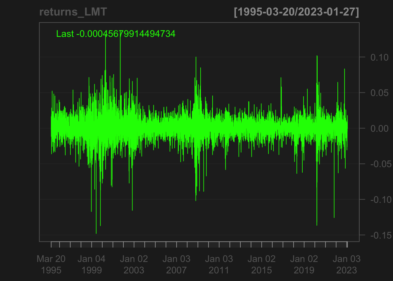

Raytheon Technologies (RTX)

Code

getSymbols("RTX", from = "1983-03-04",
           to = "2023-01-30", src="yahoo")

[1] "RTX"

Code

rtx.close<- Ad(RTX)
returns_RTX = diff(log(rtx.close))
chartSeries(returns_RTX)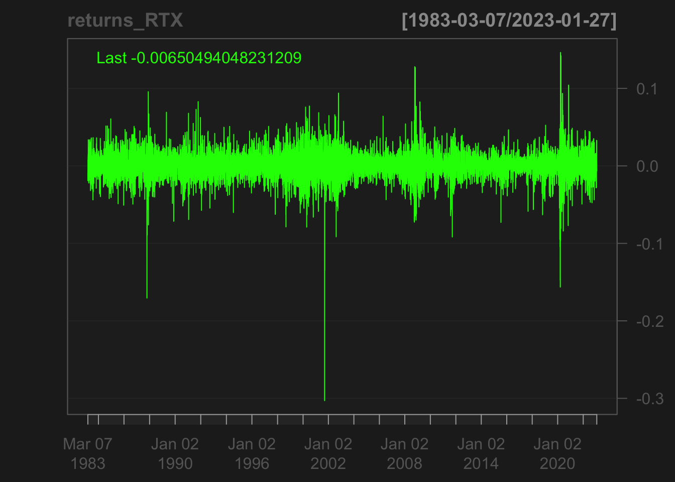

Dow Jones U.S. Travel & Tourism Index (DJUSTT)

Code

getSymbols("^DJUSTT", from = "2008-12-01",
           to = "2023-01-30", src="yahoo")

[1] "^DJUSTT"

Code

djustt.close<- Ad(DJUSTT)
returns_DJUSTT = diff(log(djustt.close))
chartSeries(returns_DJUSTT)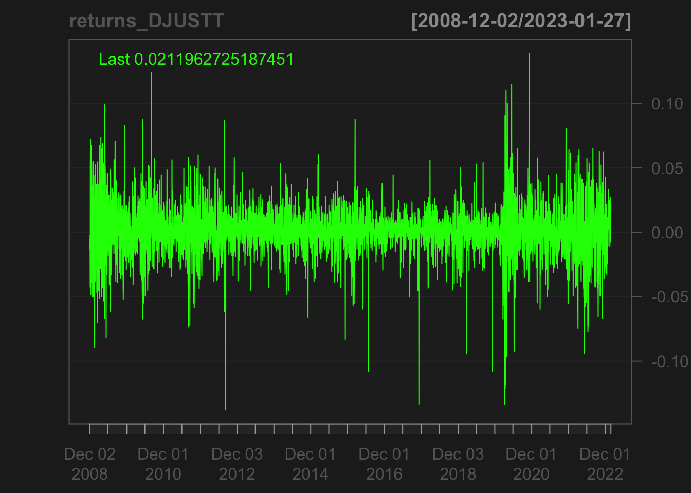

Lockheed Martin (LMT): The candlestick chart for LMT shows a predominantly bullish trend, with a series of higher highs and higher lows over the course of the time period. There are a few instances of short-term bearish reversals, but overall the stock appears to be in an upward trend. The shadows of the candlesticks are generally small, indicating relatively little price volatility, but there are a few instances of longer shadows, which may be a sign of increased uncertainty or volatility.

LMT’s returns does support the findings from the candlestick chart. We see evidence of volatility clustering during three distinct periods: around 1998-2000, the beginning of 2009-2010, and the beginning of 2020 to the end of 2021. This clustering of volatility is consistent with the findings of many financial studies, and can have important implications for trading strategies and risk management. One approach to modeling volatility clustering is to use ARCH/GARCH models, which are specifically designed to capture the time-varying volatility of financial time series data.

In the case of LMT, we can use the candlestick chart to gain additional insights into these periods of volatility clustering. For example, during the period from 1998-2000, we can see that there are several long shadows and a few bearish engulfing patterns, which may have contributed to the increased volatility during that time period. Similarly, during the beginning of 2009-2010 and the beginning of 2020 to the end of 2021, we can see that the candlestick chart shows increased uncertainty and volatility, with larger and more frequent bullish and bearish candlesticks.

By using ARCH/GARCH models to model the time-varying volatility of LMT returns, we can gain a more accurate understanding of the underlying dynamics of the stock’s behavior, and potentially identify trading opportunities or develop more effective risk management strategies.

Raytheon Technologies (RTX): The candlestick chart for RTX shows a more mixed trend, with periods of both bullish and bearish behavior over the time period. There are several instances of long shadows, indicating significant price volatility, particularly in the early part of the time period. The candlesticks also show several instances of short-term reversals, with a few examples of bearish engulfing patterns, which may be a cause for concern for investors. Although RTX also shows evidence of volatility clustering during three distinct periods - January 1998, December 2000, and January 2019 - it is far less volatile compared to LMT. The candlestick chart for RTX reveals that during these periods, there were some large bullish and bearish candlesticks but not as frequent or as large as in the case of LMT.

The low volatility of RTX may suggest that it could be a more stable investment option compared to LMT, but it is important to note that low volatility can also lead to lower returns. Additionally, the volatility clustering observed in RTX may still pose a risk for investors who are not adequately prepared to manage the potential impact of unexpected market events.

The use of ARCH/GARCH models may help us understand the underlying dynamics of RTX’s returns, despite its low volatility. By modeling the time-varying volatility of RTX returns, we can potentially identify periods of heightened risk and better manage our investment strategy accordingly.

The candlestick chart can also provide additional insights into these periods of volatility clustering. For instance, during Jan 1998 and December 2000, we can see that there were several long shadows and a few bearish engulfing patterns, indicating a shift in sentiment towards selling. Similarly, in January 2019, we can see some long bullish candlesticks, which suggest a bullish sentiment among investors. These patterns can be useful for developing trading strategies and for understanding market sentiment.

Dow Jones Travel and Tourism Index (DJUSTT): The candlestick chart for the DJTTRX shows a predominantly bullish trend, with a steady increase in price over the course of the time period. There are a few instances of short-term bearish reversals, but overall the trend is upward. The shadows of the candlesticks are generally small, indicating relatively little price volatility, but there are a few instances of longer shadows, which may be a sign of increased uncertainty or volatility. It’s also worth noting that the trend appears to be accelerating in the latter part of the time period, with more frequent and larger bullish candlesticks.

The candlestick analysis of DJUSTT reveals a consistent pattern of volatility clustering, which is also evident in its returns. The ARCH/GARCH models can be used to capture the clustering of volatility in DJUSTT’s returns. The clusters of high volatility are reflected in the candlestick chart as long candlesticks, indicating large price movements. The GARCH model can help identify periods of high volatility and provide insight into the potential future volatility of DJUSTT. The presence of volatility clustering in DJUSTT’s returns suggests that market participants may be reacting to significant news or events, leading to heightened uncertainty and increased volatility. The ARCH/GARCH models can be useful tools for understanding the sources and potential impacts of such market developments, helping investors and analysts to make more informed decisions.

ACF and PACF of Returns

Lockheed Martin (LMT)

Code

returns_LMT %>% ggtsdisplay()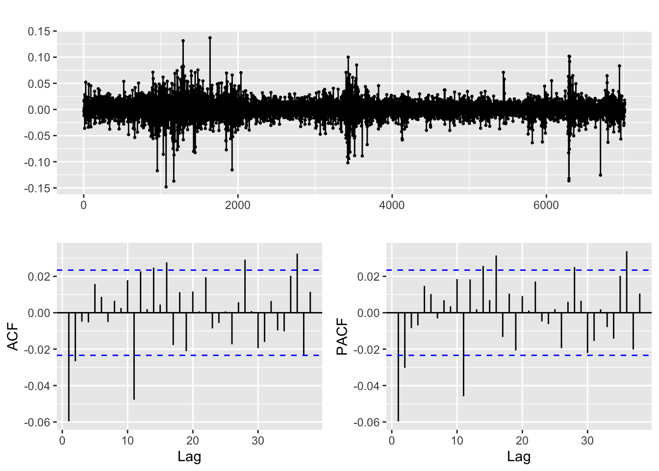 

Both ACF and PACF plots of LMT’s returns (raw) since its incorporation show high correlation, which means the series is not stationary. This may also suggest that there is strong persistence or momentum in the returns. Such patterns can be captured by ARMA models and can help to inform the selection of appropriate lag lengths for ARCH/GARCH models.

Raytheon Technologies (RTX)

Code

returns_RTX %>% ggtsdisplay() 

Like LMT’s returns, RTX’s ACF and PACF plots show high correlation, which means the series is not stationary. An AR or ARMA model might be required to fit the series before fitting the ARCH/GARCH model.

Dow Jones Travel and Tourism Index (DJUSTT)

Code

returns_DJUSTT %>% ggtsdisplay()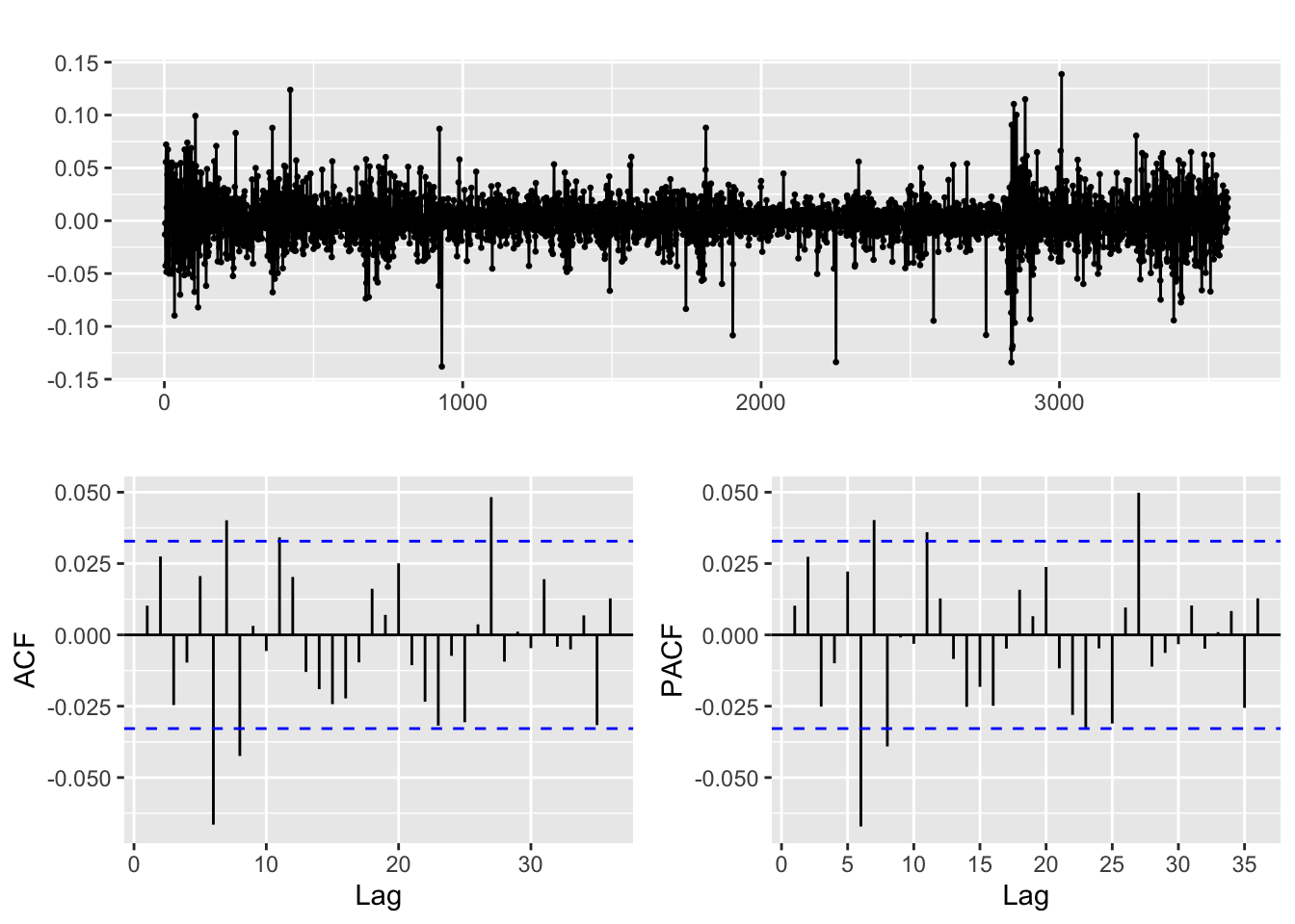 

The ACF and PACF plots of DJUSTT returns suggest that there may be some autocorrelation present in the data. Specifically, lags 1 to 5 do not appear to be significantly correlated, but there is significant autocorrelation from lag 6 onwards. This pattern of autocorrelation may be indicative of a GARCH effect, where the volatility of the series is changing over time. The presence of significant autocorrelation at higher lags may suggest that the returns exhibit a degree of persistence or momentum, where positive (or negative) returns tend to be followed by further positive (or negative) returns. Such patterns can be captured by ARMA models and can help to inform the selection of appropriate lag lengths for ARCH/GARCH models.

ACF and PACF of Squared Returns

Lockheed Martin (LMT)

Code

returns_LMT^2 %>% ggtsdisplay()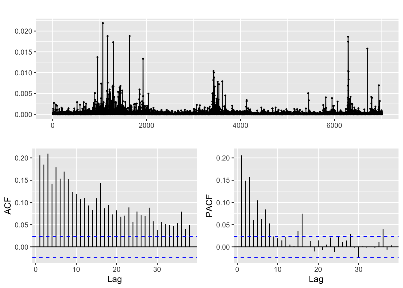 

Raytheon Technologies (RTX)

Code

returns_RTX^2 %>% ggtsdisplay() 

Dow Jones Travel and Tourism Index (DJUSTT)

Code

returns_DJUSTT^2 %>% ggtsdisplay()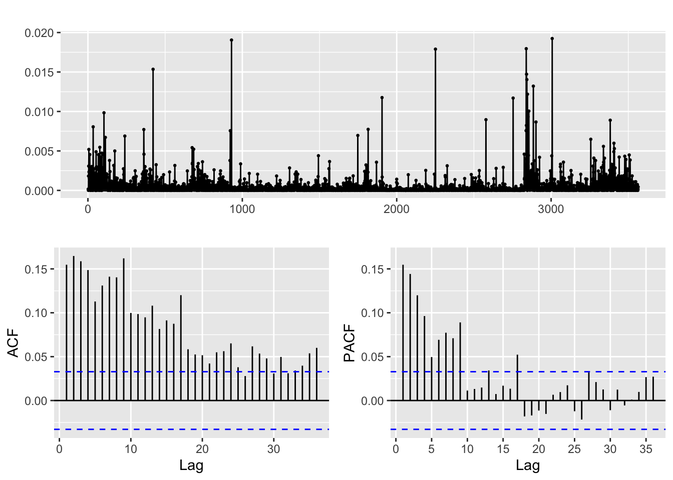 

ACF and PACF of Absolute Returns

Lockheed Martin (LMT)

Code

abs(returns_LMT) %>% ggtsdisplay()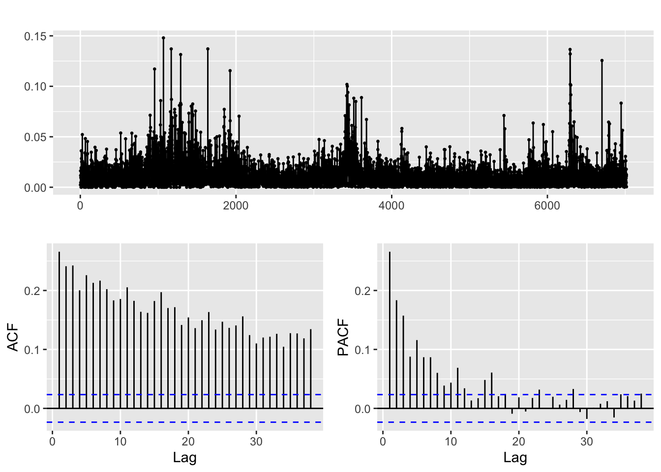 

Raytheon Technologies (RTX)

Code

abs(returns_RTX) %>% ggtsdisplay()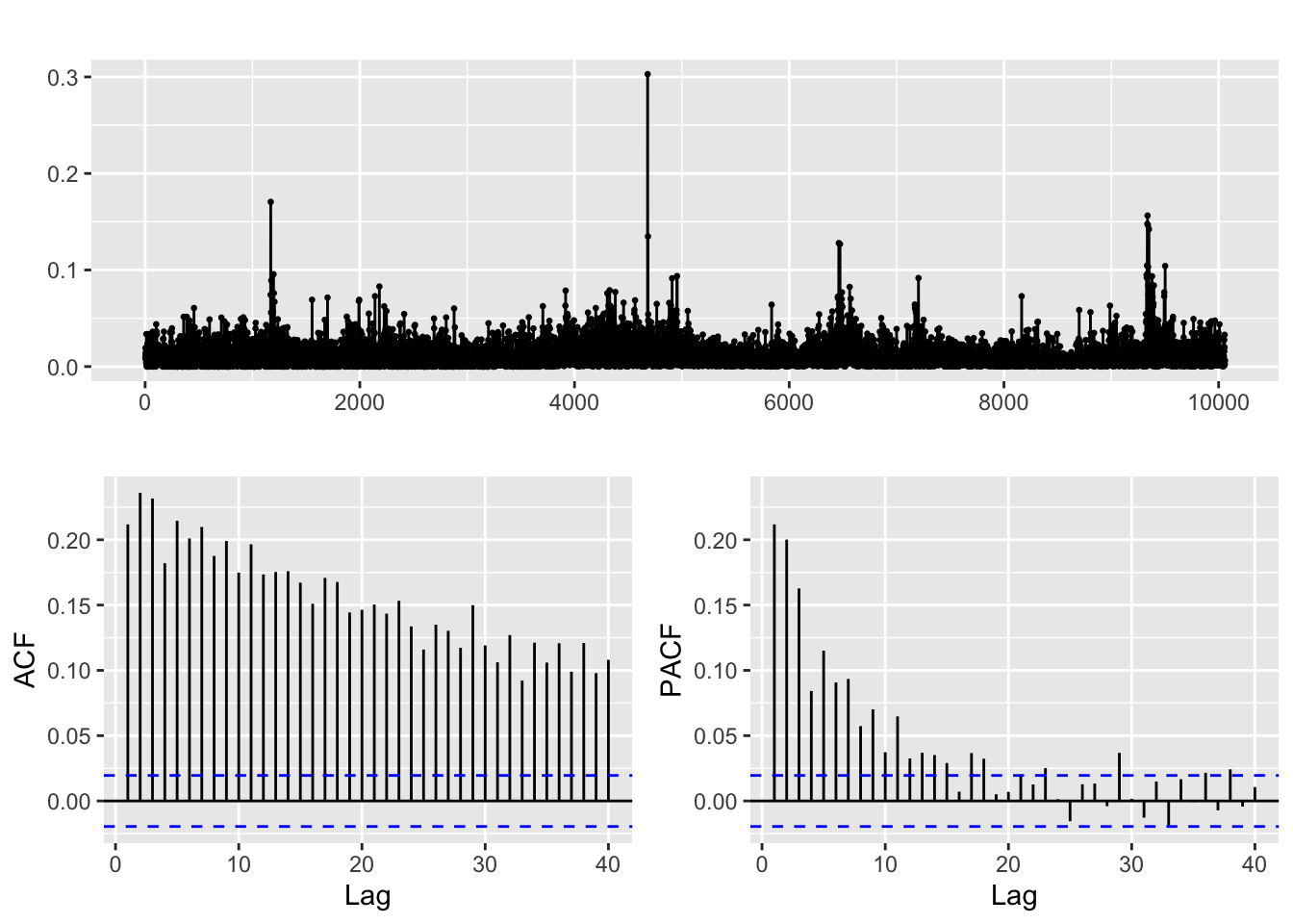 

Dow Jones Travel and Tourism Index (DJUSTT)

Code

abs(returns_DJUSTT) %>% ggtsdisplay()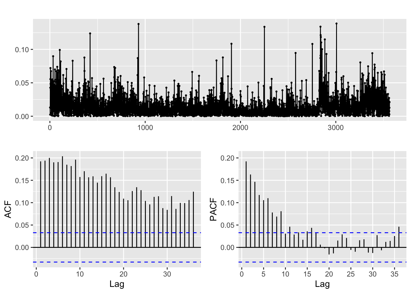 

After transforming the returns, clear correlation is discerned in both ACF and PACF plots for all three financial series when we examine their absolute and squared returns. It is likely that there is some non-linear dependence present in the data, which could be attributed to volatility clustering, signifying periods of high volatility tend to be followed by periods of high volatility, and periods of low volatility tend to be followed by periods of low volatility. This pattern can be captured by ARCH/GARCH models, which allow for the conditional variance of the series to depend on past squared returns. The decreasing significance of the ACF and PACF at higher lags may indicate that the effects of past volatility on current volatility decay over time, which can be modeled by including lagged terms of the conditional variance in the ARCH/GARCH models. Overall, the ACF and PACF plots of squared returns can provide useful information about the structure of the data and can guide the development of appropriate time series models for capturing the volatility clustering.

Therefore, just fitting an ARCH model to each series is not enough! An ARCH model, which is designed to capture volatility clustering or autocorrelation in the squared returns, could be a good starting point. However, an ARCH model only models the conditional variance of the data and assumes that the conditional mean is constant over time. Since there is also autocorrelation in the returns themselves, then an ARMA or ARIMA model may be necessary to model the conditional mean. Therefore, we should fit an ARMA or ARIMA model first to the stocks and then fit an ARCH to the residuals of the ARMA or ARIMA model.

Fitting ARIMA Model

ACF and PACF of Lockheed Martin (LMT) Stock’s Transformations (Log, Difference, Differenced Log)

Log Transformation

Code

log.lmt=log(lmt.close)

log.lmt %>% ggtsdisplay()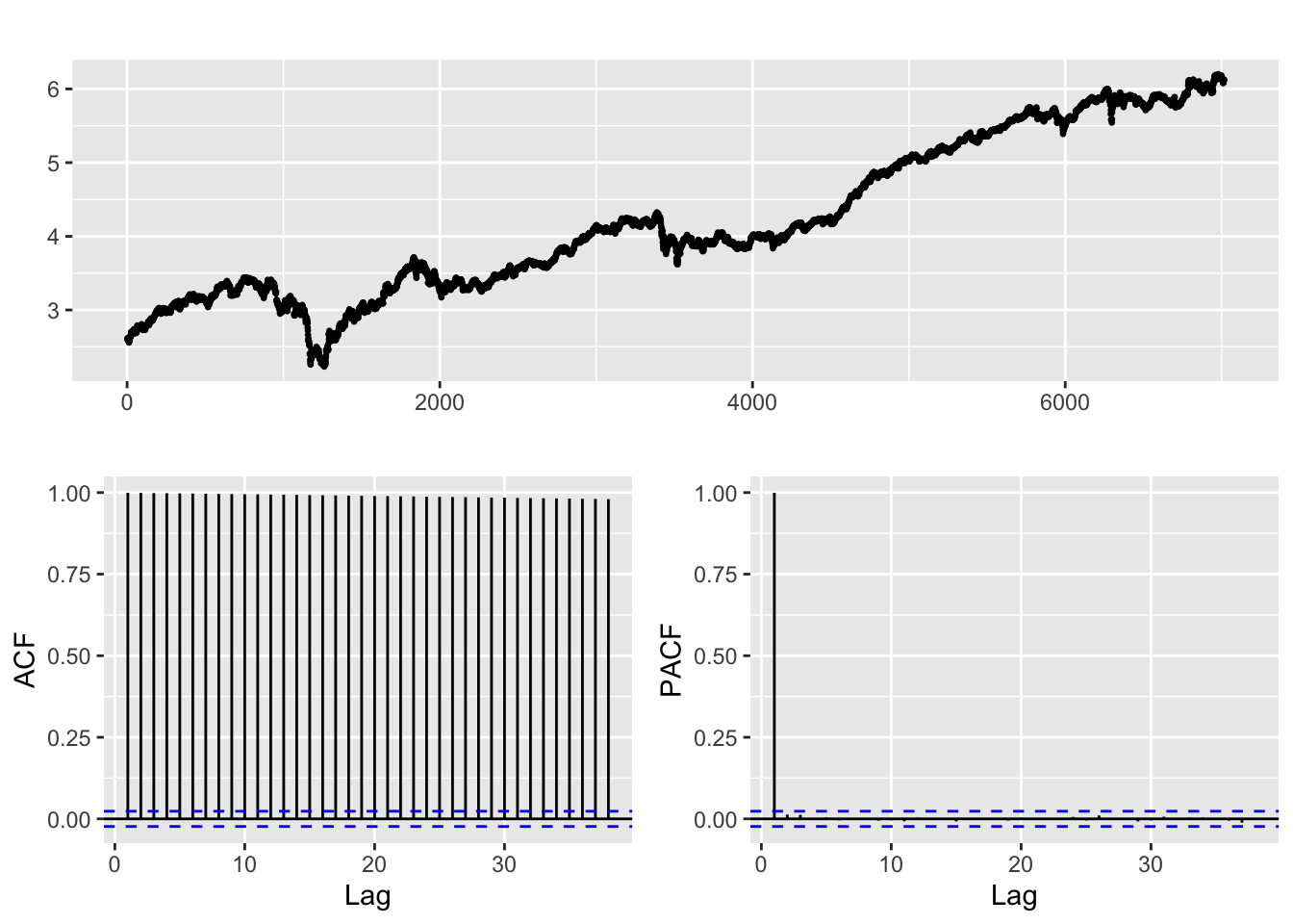

Differenced Transformation

Code

diff.lmt=diff(lmt.close)

diff.lmt %>% ggtsdisplay()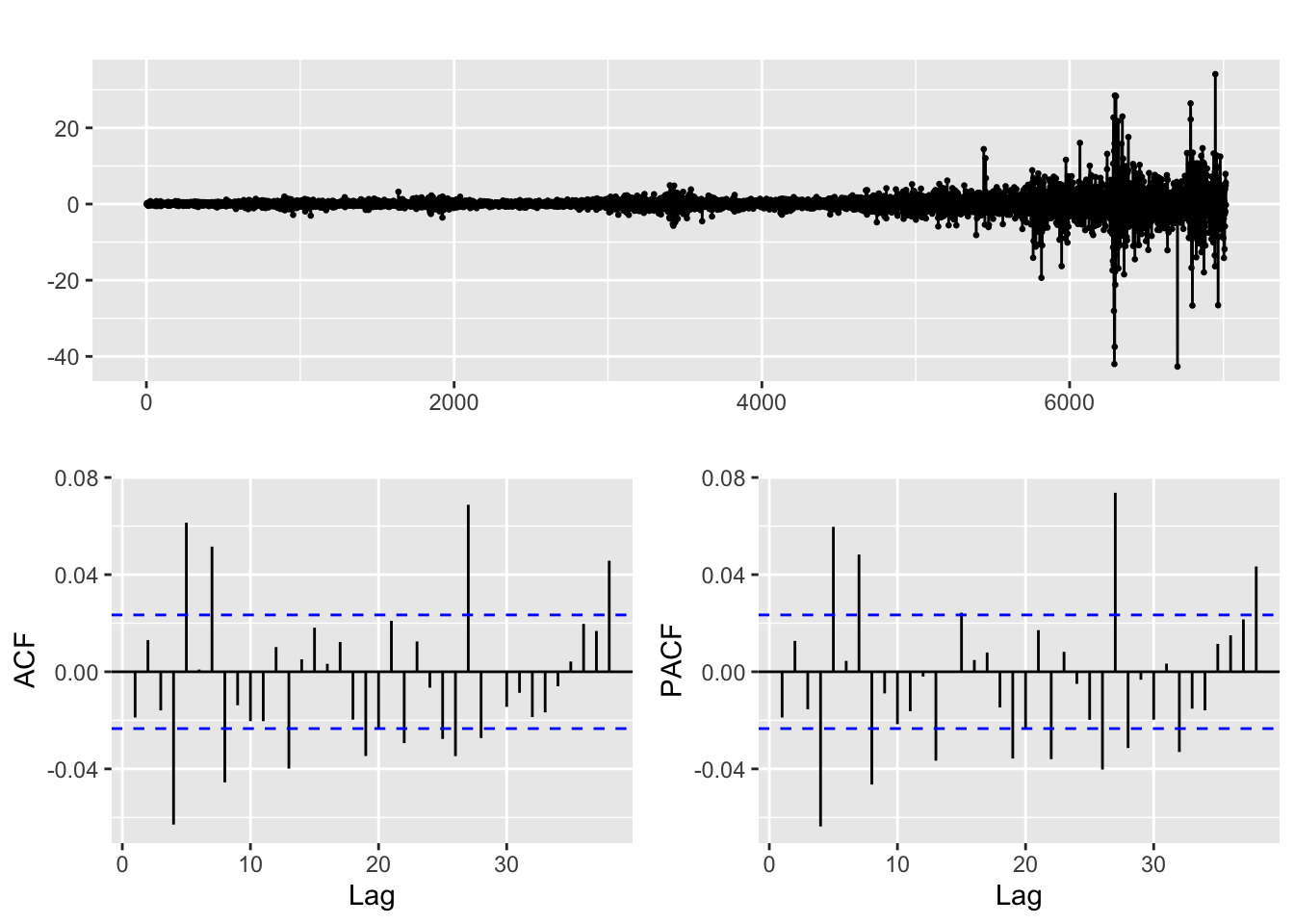

Differenced Log Transformation

Code

logdiff.lmt=diff(log(lmt.close))

logdiff.lmt %>% ggtsdisplay()

Only when LMT is transformed by both differencing and taking the log of its stock price, we obtain a weakly stationary series, not otherwise. The model for “differenced log LMT” series is a white noise, and the “original model” resembles random walk model ARIMA(0,1,0). Therefore, we shall fit an ARIMA(p,1,d) model to its log price.

ACF and PACF of Raytheon Technologies (RTX) Stock’s Transformations (Log, Difference, Differenced Log)

Log Transformation

Code

log.rtx=log(rtx.close)

log.rtx %>% ggtsdisplay()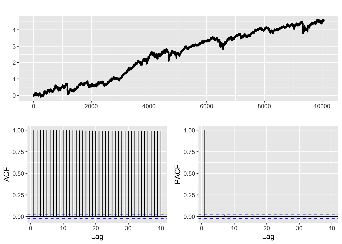

Differenced Transformation

Code

diff.rtx=diff(rtx.close)

diff.rtx %>% ggtsdisplay()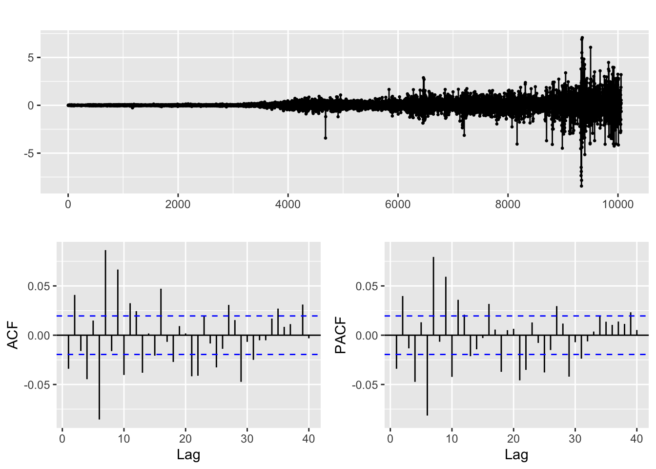

Differenced Log Transformation

Code

difflog.rtx=diff(log(rtx.close))

difflog.rtx %>% ggtsdisplay()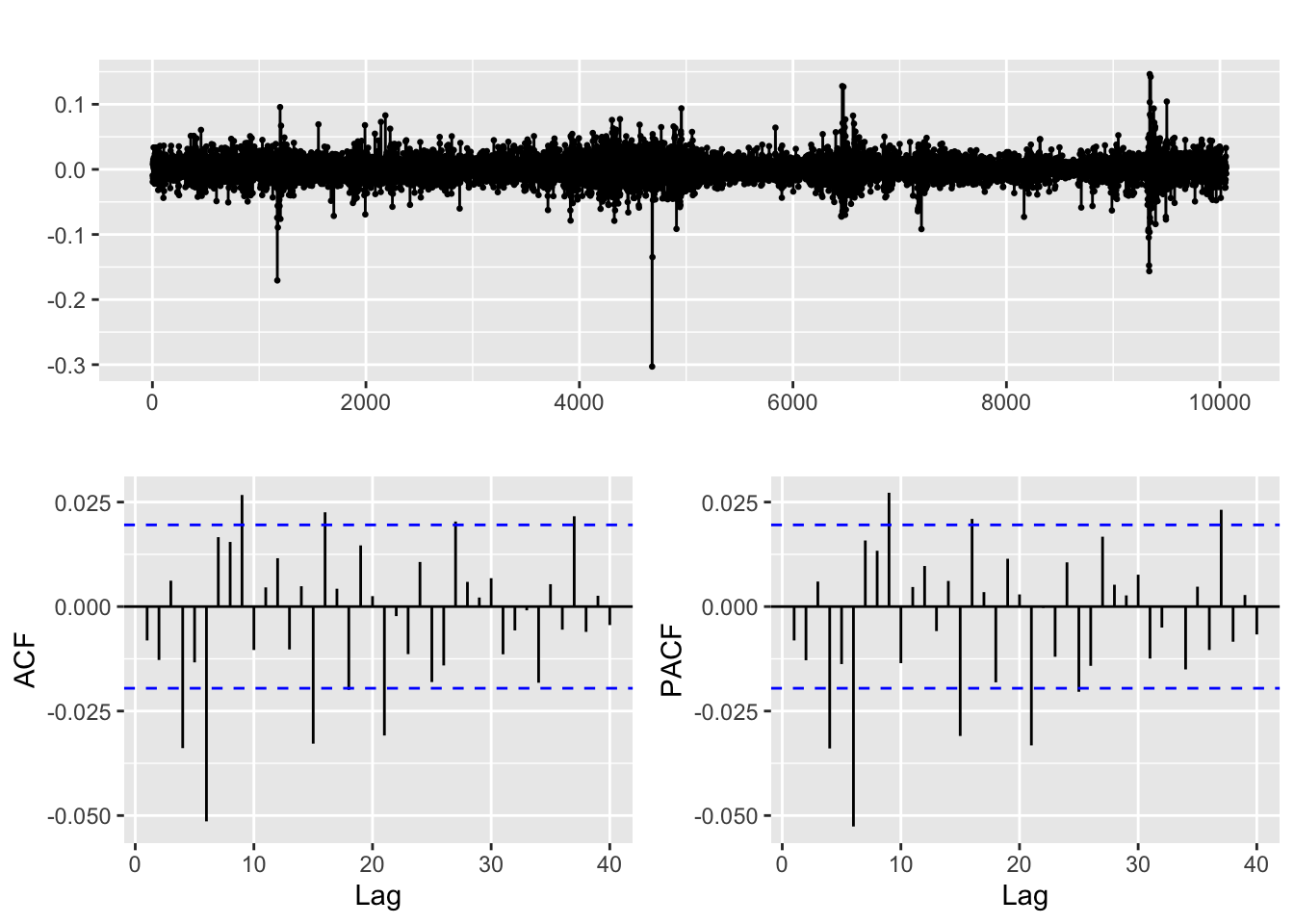

The same is true for RTX’s stock price, both differencing and taking the log of its stock price gives us a weakly stationary series.

ACF and PACF of Dow Jones Travel and Tourism Index’s (DJUSTT) Transformations (Log, Difference, Differenced Log)

Log Transformation

Code

log.djustt=log(djustt.close)

log.djustt %>% ggtsdisplay()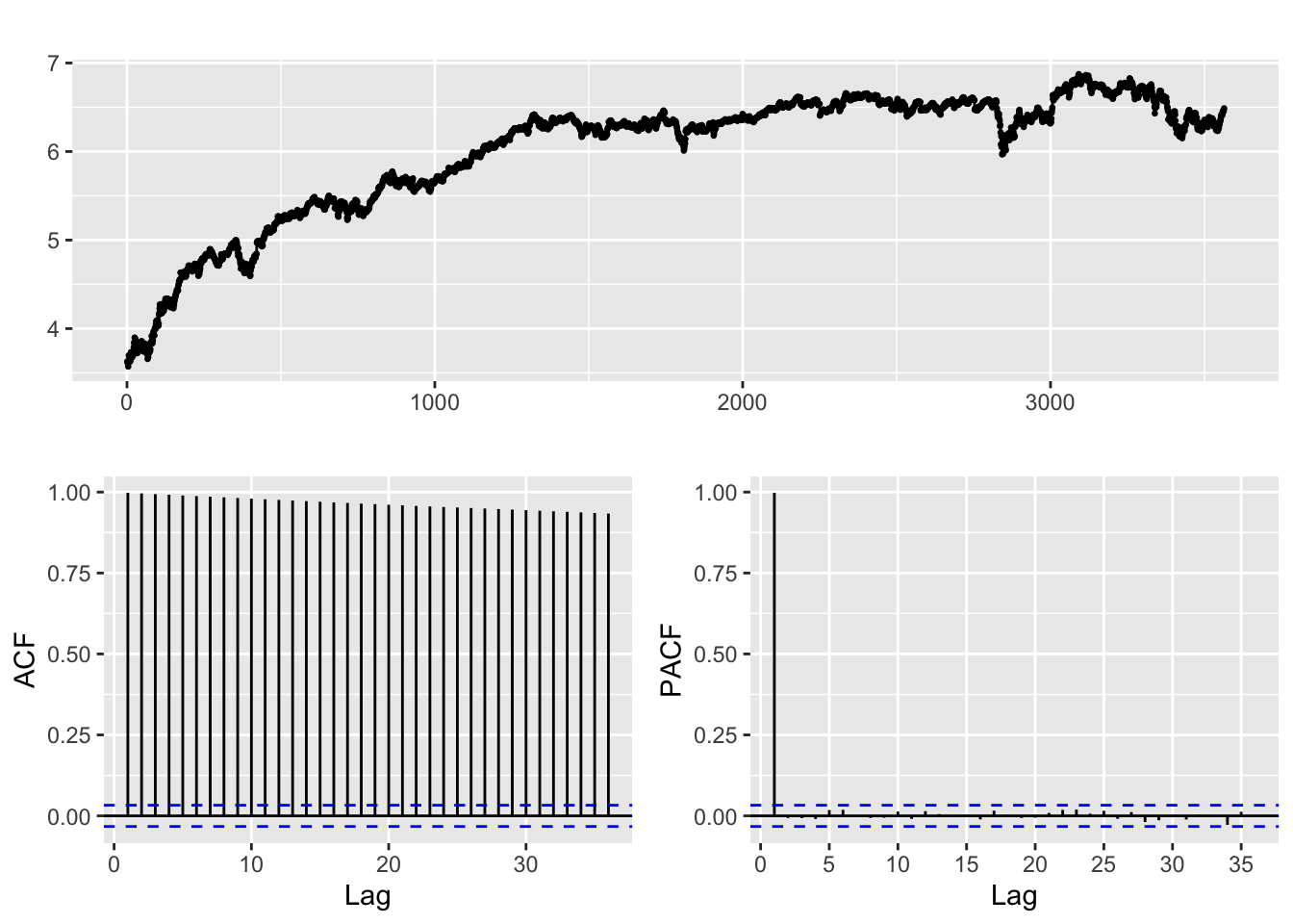

Differenced Transformation

Code

diff.djustt=diff(djustt.close)

diff.djustt %>% ggtsdisplay()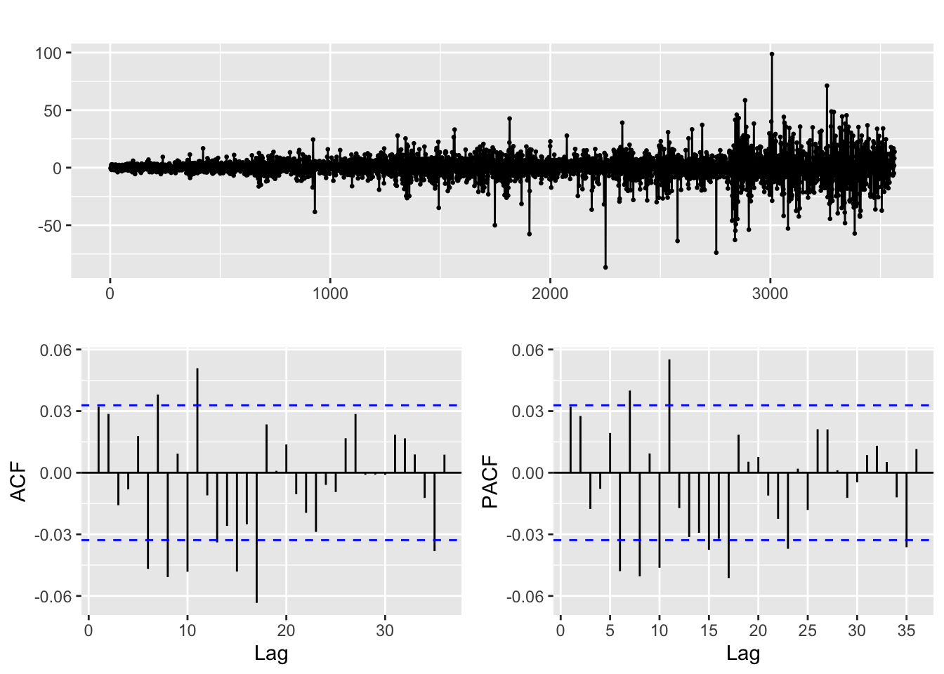

Differenced Log Transformation

Code

logdiff.djustt=log(diff(djustt.close))

logdiff.djustt %>% ggtsdisplay()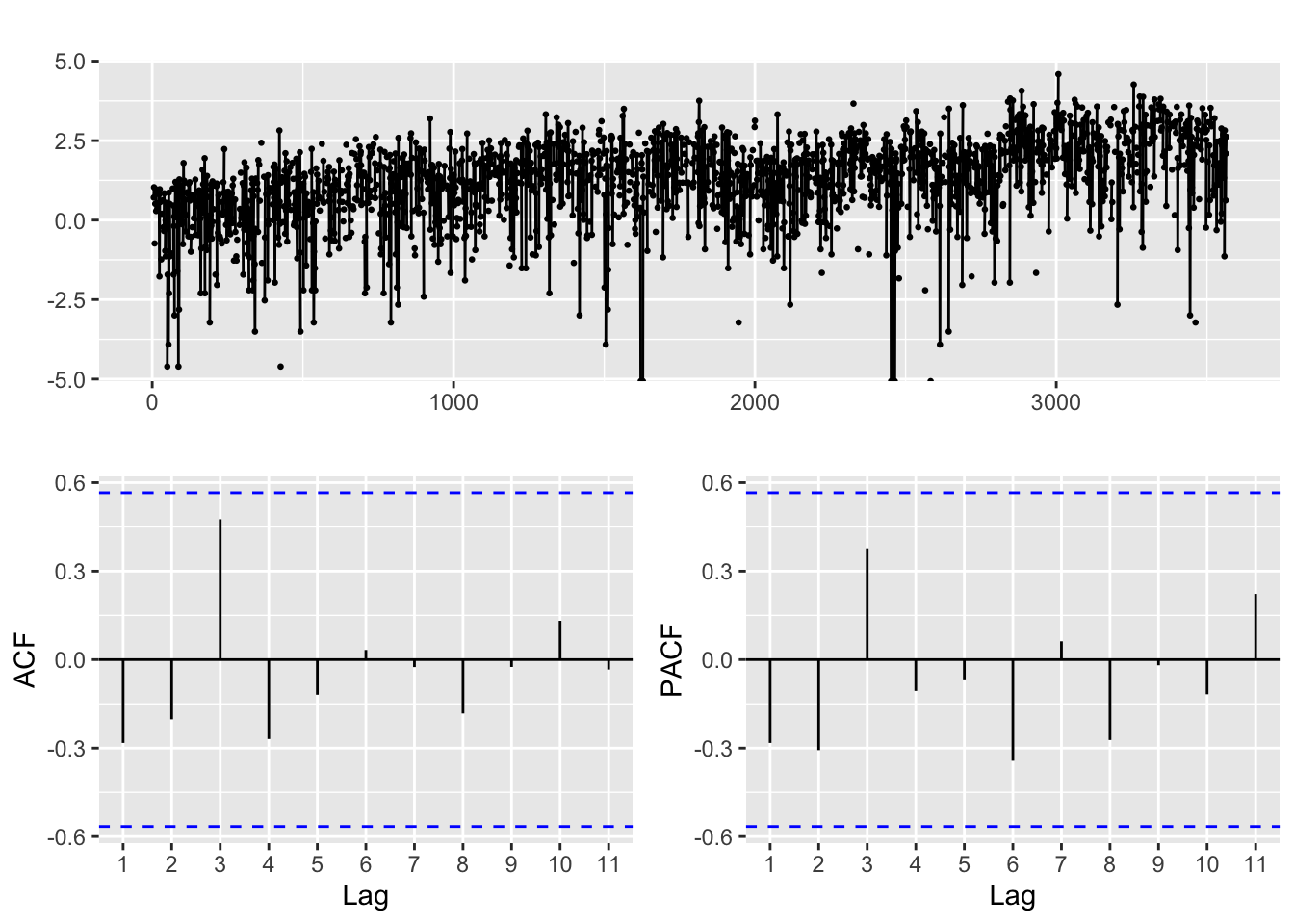

Differencing and taking the log of the index leads to a stationary series, unlike the weakly stationary series obtained from both stocks.

Checking for different ARIMA(p,q,d) Combinations: Lockheed Martin (LMT)

Code

######################## Check for different combinations ########


d=1
i=1
temp= data.frame()
ls=matrix(rep(NA,6*32),nrow=32) # roughly nrow = 3x4x2


for (p in 1:4)# p=1,2,3
{
  for(q in 1:4)# q=1,2,3
  {
    for(d in 0:1)
    {
      
      if(p-1+d+q-1<=8)
      {
        
        model<- Arima(log.lmt,order=c(p-1,d,q-1),include.drift=TRUE) 
        ls[i,]= c(p-1,d,q-1,model$aic,model$bic,model$aicc)
        i=i+1
        #print(i)
        
      }
      
    }
  }
}

temp= as.data.frame(ls)
names(temp)= c("p","d","q","AIC","BIC","AICc")

#temp
knitr::kable(temp)

p	d	q	AIC	BIC	AICc
0	0	0	3286.409	3306.977	3286.412
0	1	0	-37587.582	-37573.870	-37587.580
0	0	1	-5825.116	-5797.692	-5825.110
0	1	1	-37612.101	-37591.534	-37612.098
0	0	2	-13119.176	-13084.896	-13119.167
0	1	2	-37615.382	-37587.958	-37615.376
0	0	3	-18328.549	-18287.414	-18328.537
0	1	3	-37613.519	-37579.240	-37613.511
1	0	0	-37589.010	-37561.586	-37589.004
1	1	0	-37610.570	-37590.003	-37610.567
1	0	1	-37612.881	-37578.601	-37612.872
1	1	1	-37615.042	-37587.619	-37615.037
1	0	2	-37615.912	-37574.776	-37615.900
1	1	2	-37613.325	-37579.046	-37613.317
1	0	3	-37614.017	-37566.025	-37614.001
1	1	3	-37611.513	-37570.378	-37611.501
2	0	0	-37611.418	-37577.138	-37611.409
2	1	0	-37614.998	-37587.575	-37614.993
2	0	1	-37615.260	-37574.124	-37615.248
2	1	1	-37613.106	-37578.827	-37613.098
2	0	2	-37614.875	-37566.883	-37614.859
2	1	2	-37611.501	-37570.366	-37611.489
2	0	3	-37611.913	-37557.066	-37611.893
2	1	3	-37609.506	-37561.515	-37609.490
3	0	0	-37615.580	-37574.444	-37615.568
3	1	0	-37613.493	-37579.214	-37613.484
3	0	1	-37612.079	-37564.087	-37612.063
3	1	1	-37611.517	-37570.382	-37611.505
3	0	2	-37611.934	-37557.087	-37611.914
3	1	2	-37609.526	-37561.535	-37609.510
3	0	3	-37610.049	-37548.345	-37610.023
3	1	3	-37607.518	-37552.671	-37607.497

Code

cat("Lowest AIC model: \n")

Lowest AIC model: 

Code

temp[which.min(temp$AIC),] # 0,1,0

   p d q       AIC       BIC     AICc
13 1 0 2 -37615.91 -37574.78 -37615.9

Code

cat("\nLowest BIC model: \n")

Lowest BIC model: 

Code

temp[which.min(temp$BIC),] # 0,1,1

  p d q      AIC       BIC     AICc
4 0 1 1 -37612.1 -37591.53 -37612.1

Code

cat("\nLowest AICc model: \n")

Lowest AICc model: 

Code

temp[which.min(temp$AICc),] # 0,1,0

   p d q       AIC       BIC     AICc
13 1 0 2 -37615.91 -37574.78 -37615.9

We shall choose ARIMA(0,1,1) as the best model for LMT, given it has the lowest BIC, its AIC is fairly close to other, more complex ARIMA model, ARIMA(1,0,2) or ARMA(1,2), and we shall be abiding by the principle of parsimony. Moreover, an ARMA model only captures the conditional mean, whereas an ARIMA model captures both the conditional mean and conditional variance.

Checking for different ARIMA(p,q,d) Combinations: Raytheon Technologies (RTX)

Code

######################## Check for different combinations ########


d=1
i=1
temp= data.frame()
ls=matrix(rep(NA,6*32),nrow=32) # roughly nrow = 3x4x2


for (p in 1:4)# p=1,2,3
{
  for(q in 1:4)# q=1,2,3
  {
    for(d in 0:1)
    {
      
      if(p-1+d+q-1<=8)
      {
        
        model<- Arima(log.rtx,order=c(p-1,d,q-1),include.drift=TRUE) 
        ls[i,]= c(p-1,d,q-1,model$aic,model$bic,model$aicc)
        i=i+1
        #print(i)
        
      }
      
    }
  }
}

temp= as.data.frame(ls)
names(temp)= c("p","d","q","AIC","BIC","AICc")

#temp
knitr::kable(temp)

p	d	q	AIC	BIC	AICc
0	0	0	2907.649	2929.298	2907.652
0	1	0	-53301.081	-53286.648	-53301.079
0	0	1	-10229.369	-10200.504	-10229.365
0	1	1	-53299.758	-53278.110	-53299.756
0	0	2	-20271.791	-20235.710	-20271.785
0	1	2	-53299.498	-53270.633	-53299.494
0	0	3	-27788.091	-27744.794	-27788.083
0	1	3	-53297.809	-53261.728	-53297.803
1	0	0	-53306.312	-53277.448	-53306.308
1	1	0	-53299.741	-53278.092	-53299.738
1	0	1	-53304.842	-53268.761	-53304.836
1	1	1	-53297.750	-53268.885	-53297.746
1	0	2	-53304.339	-53261.042	-53304.330
1	1	2	-53297.504	-53261.423	-53297.498
1	0	3	-53302.780	-53252.266	-53302.769
1	1	3	-53295.827	-53252.530	-53295.818
2	0	0	-53304.829	-53268.748	-53304.823
2	1	0	-53299.400	-53270.535	-53299.396
2	0	1	-53309.025	-53265.728	-53309.017
2	1	1	-53297.394	-53261.313	-53297.388
2	0	2	-53313.402	-53262.889	-53313.391
2	1	2	-53309.650	-53266.354	-53309.642
2	0	3	-53312.564	-53254.834	-53312.549
2	1	3	-53308.589	-53258.076	-53308.578
3	0	0	-53304.259	-53260.962	-53304.251
3	1	0	-53297.760	-53261.680	-53297.755
3	0	1	-53313.566	-53263.053	-53313.555
3	1	1	-53295.746	-53252.449	-53295.738
3	0	2	-53310.859	-53253.129	-53310.844
3	1	2	-53309.273	-53258.760	-53309.262
3	0	3	-53310.162	-53245.216	-53310.144
3	1	3	-53318.139	-53260.410	-53318.124

Code

cat("Lowest AIC model: \n")

Lowest AIC model: 

Code

temp[which.min(temp$AIC),] # 3,1,3

   p d q       AIC       BIC      AICc
32 3 1 3 -53318.14 -53260.41 -53318.12

Code

cat("\nLowest BIC model: \n")

Lowest BIC model: 

Code

temp[which.min(temp$BIC),] # 0,1,0

  p d q       AIC       BIC      AICc
2 0 1 0 -53301.08 -53286.65 -53301.08

Code

cat("\nLowest AICc model: \n")

Lowest AICc model: 

Code

temp[which.min(temp$AICc),] # 3,1,3

   p d q       AIC       BIC      AICc
32 3 1 3 -53318.14 -53260.41 -53318.12

We shall choose ARIMA(0,1,0), a random walk, as the best model for RTX, given it has the lowest BIC, its AIC is fairly close to other, more complex ARIMA model, ARIMA(3,1,3), and we shall be abiding by the principle of parsimony.

Checking for different ARIMA(p,q,d) Combinations: Dow Jones Travel and Tourism Index (DJUSTT)

Code

######################## Check for different combinations ########


d=1
i=1
temp= data.frame()
ls=matrix(rep(NA,6*32),nrow=32) # roughly nrow = 3x4x2


for (p in 1:4)# p=1,2,3
{
  for(q in 1:4)# q=1,2,3
  {
    for(d in 0:1)
    {
      
      if(p-1+d+q-1<=8)
      {
        
        model<- Arima(djustt.close,order=c(p-1,d,q-1),include.drift=TRUE) # taking log gives NA error (dont want to use CSS Method that is based conditional likelihood and does not produce same likelihood value which unconditional likelihood function produces when it is optimized for the same parameters.)
        ls[i,]= c(p-1,d,q-1,model$aic,model$bic,model$aicc)
        i=i+1
        #print(i)
        
      }
      
    }
  }
}

temp= as.data.frame(ls)
names(temp)= c("p","d","q","AIC","BIC","AICc")

#temp
knitr::kable(temp)

p	d	q	AIC	BIC	AICc
0	0	0	43372.81	43391.35	43372.82
0	1	0	26850.31	26862.66	26850.31
0	0	1	38867.13	38891.84	38867.14
0	1	1	26848.82	26867.36	26848.83
0	0	2	35671.58	35702.47	35671.60
0	1	2	26847.63	26872.35	26847.64
0	0	3	33390.42	33427.49	33390.44
0	1	3	26848.56	26879.45	26848.58
1	0	0	26858.82	26883.53	26858.83
1	1	0	26848.62	26867.16	26848.63
1	0	1	26856.78	26887.67	26856.80
1	1	1	26849.44	26874.15	26849.45
1	0	2	26854.98	26892.06	26855.01
1	1	2	26849.13	26880.02	26849.15
1	0	3	26856.24	26899.49	26856.27
1	1	3	26850.55	26887.62	26850.58
2	0	0	26856.53	26887.42	26856.54
2	1	0	26847.90	26872.61	26847.91
2	0	1	26854.56	26891.63	26854.58
2	1	1	26849.43	26880.32	26849.44
2	0	2	26855.55	26898.80	26855.58
2	1	2	26848.54	26885.61	26848.57
2	0	3	26858.38	26907.80	26858.42
2	1	3	26852.44	26895.69	26852.48
3	0	0	26855.24	26892.31	26855.26
3	1	0	26848.79	26879.68	26848.81
3	0	1	26856.80	26900.05	26856.83
3	1	1	26850.81	26887.88	26850.83
3	0	2	26856.88	26906.31	26856.92
3	1	2	26852.56	26895.81	26852.59
3	0	3	26822.98	26878.59	26823.03
3	1	3	26850.58	26900.01	26850.63

Code

cat("Lowest AIC model: \n")

Lowest AIC model: 

Code

temp[which.min(temp$AIC),] # 3,0,3

   p d q      AIC      BIC     AICc
31 3 0 3 26822.98 26878.59 26823.03

Code

cat("\nLowest BIC model: \n")

Lowest BIC model: 

Code

temp[which.min(temp$BIC),] # 0,1,0

  p d q      AIC      BIC     AICc
2 0 1 0 26850.31 26862.66 26850.31

Code

cat("\nLowest AICc model: \n")

Lowest AICc model: 

Code

temp[which.min(temp$AICc),] # 3,0,3

   p d q      AIC      BIC     AICc
31 3 0 3 26822.98 26878.59 26823.03

We shall choose ARIMA(0,1,0), a random walk, as the best model for DJUSTT, given it has the lowest BIC, its AIC is fairly close to other, more complex ARIMA model, ARIMA(3,0,3), and we shall be abiding by the principle of parsimony.

Model Diagnostics

Lockheed Martin (LMT)

Code

arima.lmt=sarima(log.lmt,0,1,1)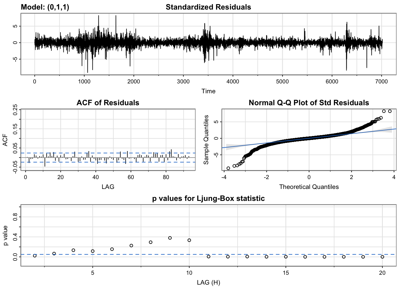

Code

summary(arima.lmt)

Raytheon Technologies (RTX)

Code

arima.rtx=sarima(log.rtx,0,1,0)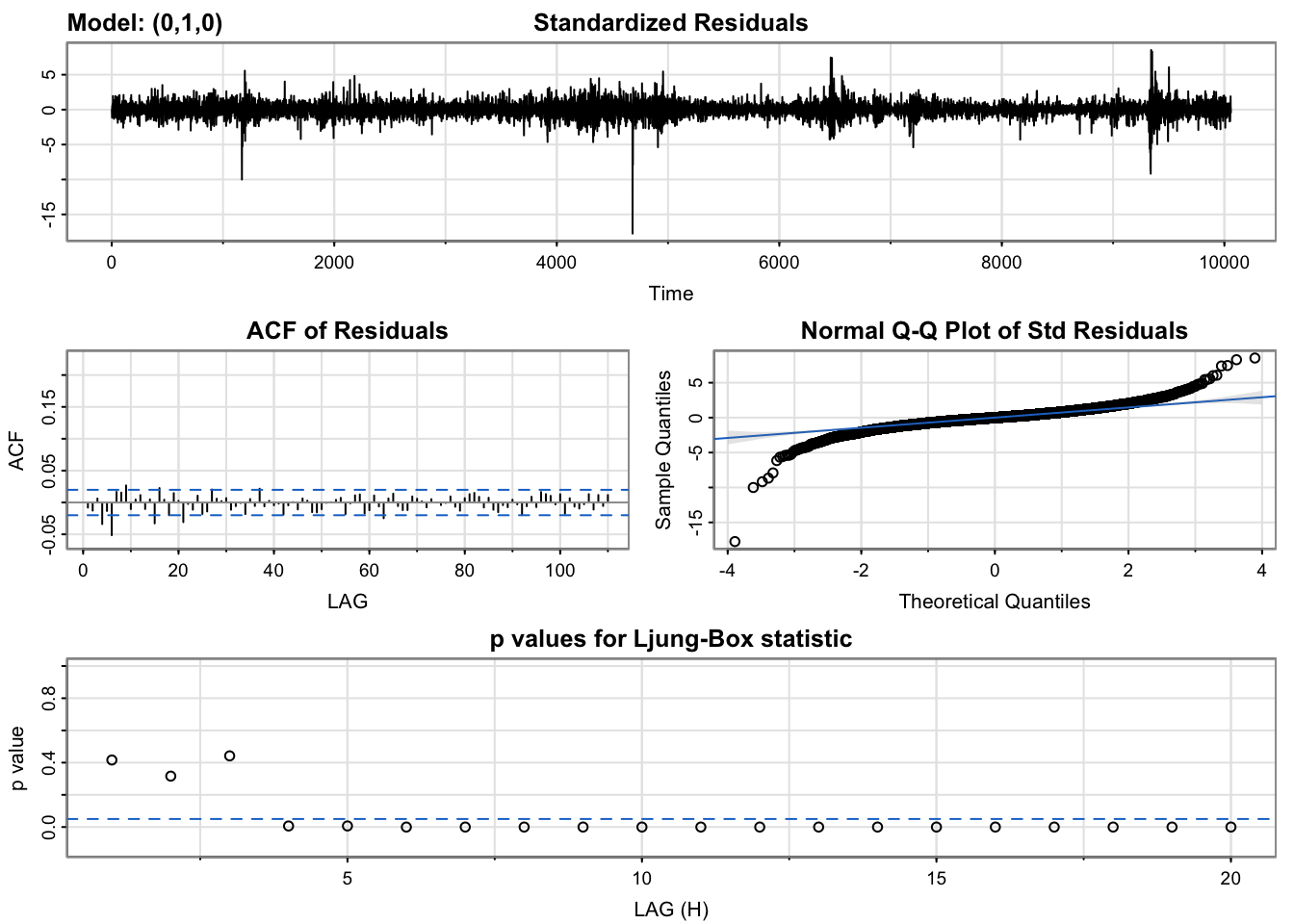

Code

summary(arima.rtx)

Dow Jones Travel and Tourism Index (DJUSTT)

Code

arima.djustt=sarima(djustt.close,0,1,0)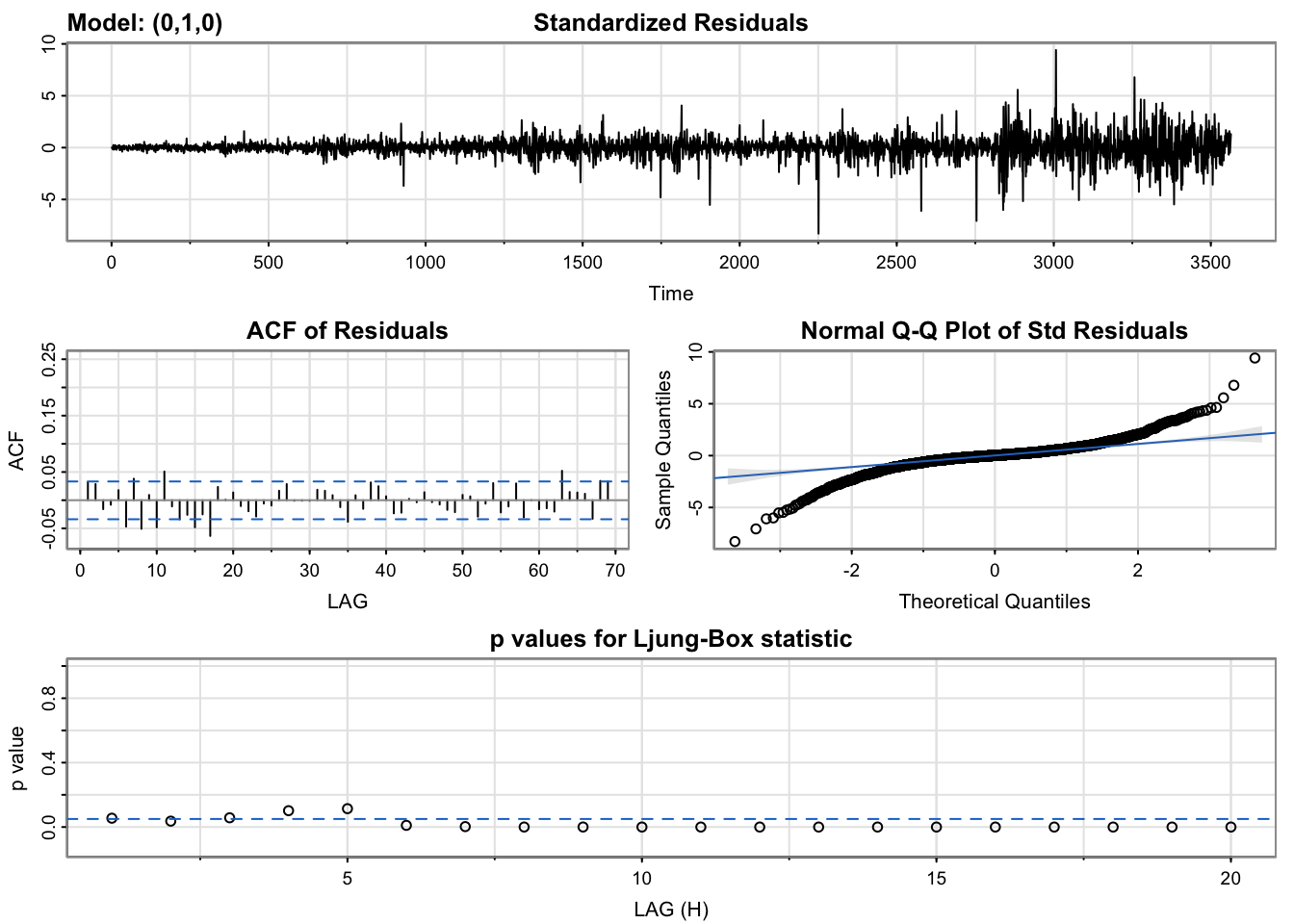

Code

summary(arima.djustt)

Lockheed Martin (LMT):

The plot of standardized residuals should have a mean around 0 and a variance of approximately 1. The plot for LMT generally meets the criterion for the mean but has higher variance with clusters, indicating the need for an ARCH/GARCH model for the errors. The absence of significant lags in the ACF plot of residuals is an encouraging sign. The qq-plot indicates some signs of normality with slight skew at the tails. In addition, the p-values for the Ljung-Box test are above 0.05 for many lags, suggesting a well-fitted model. Ideally, we would like to fail to reject the null hypothesis. That is, we would like to see the p-value of the test be greater than 0.05 because this means the residuals for our time series model are independent. Overall, while the variance of the standardized residuals suggests the need for an ARCH/GARCH model, the other diagnostic plots indicate a good fit for the ARIMA model.

Raytheon Technologies (RTX):

The plot of standardized residuals for RTX is also centered around 0 and has significantly lower number of clusters. Moreover, the variance within those few clusters is not as high as those in LMT’s plot of standardized residuals. In addition, the p-values for the Ljung-Box test are above 0.05 for the first few lags and the absence of significant lags in the ACF plot of residuals is an encouraging sign. The qq-plot indicates some signs of normality with slight skew at the tails.

Dow Jones Travel and Tourism Index (DJUSTT):

The plot of standardized residuals for RTX is also centered around 0 and has significantly lower number of clusters. Moreover, the variance within those few clusters is not as high as those in LMT’s plot of standardized residuals. Although none of the p-values for the Ljung-Box test are above 0.05, signifying that the residuals might not be independently distributed or that they exhibit serial correlation, a random walk model can be expected to show these outputs. Regardless, the absence of significant lags in the ACF plot of residuals is an encouraging sign. The qq-plot indicates some signs of normality with slight skew at the tails.

Plotting Squared Residuals of Chosen Models and their ACFs and PACFs

Lockheed Martin (LMT)

Code

arima.lmt=Arima(log.lmt,order=c(0,1,1))
res.arima.lmt=arima.lmt$res
sq.res.arima.lmt=res.arima.lmt^2

sq.res.arima.lmt %>% ggtsdisplay()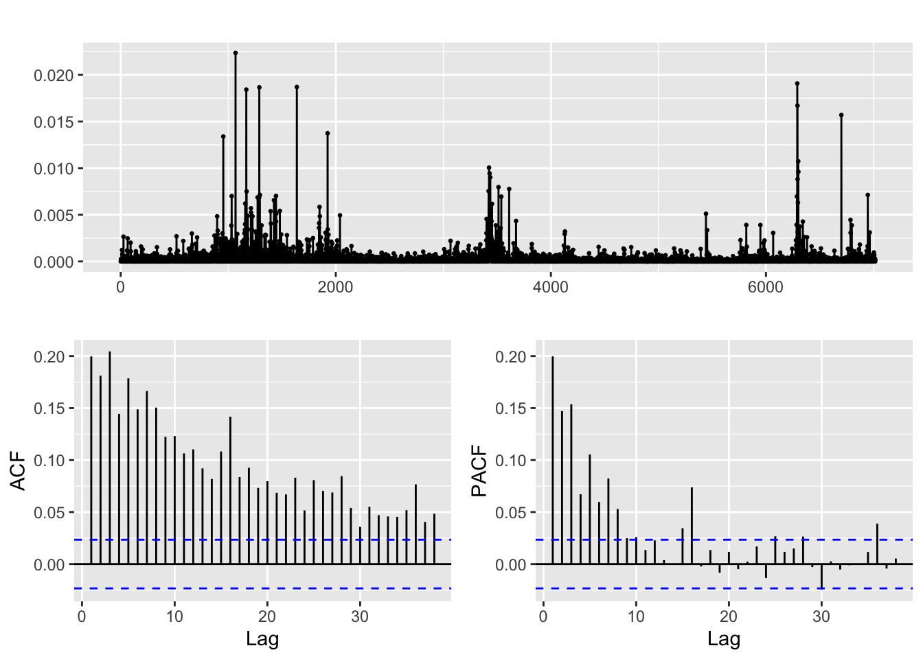

Raytheon Technologies (RTX)

Code

arima.rtx=Arima(log.rtx,order=c(0,1,0))
res.arima.rtx=arima.rtx$res
sq.res.arima.rtx=res.arima.rtx^2

sq.res.arima.rtx %>% ggtsdisplay()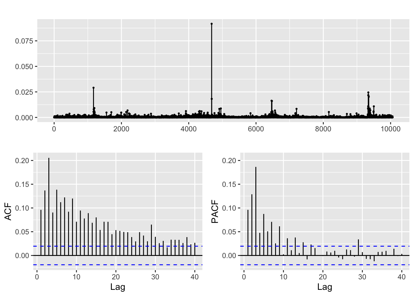

Dow Jones Travel and Tourism Index (DJUSTT)

Code

arima.djustt=Arima(djustt.close,order=c(0,1,0))
res.arima.djustt=arima.djustt$res
sq.res.arima.djustt=res.arima.djustt^2

sq.res.arima.djustt %>% ggtsdisplay()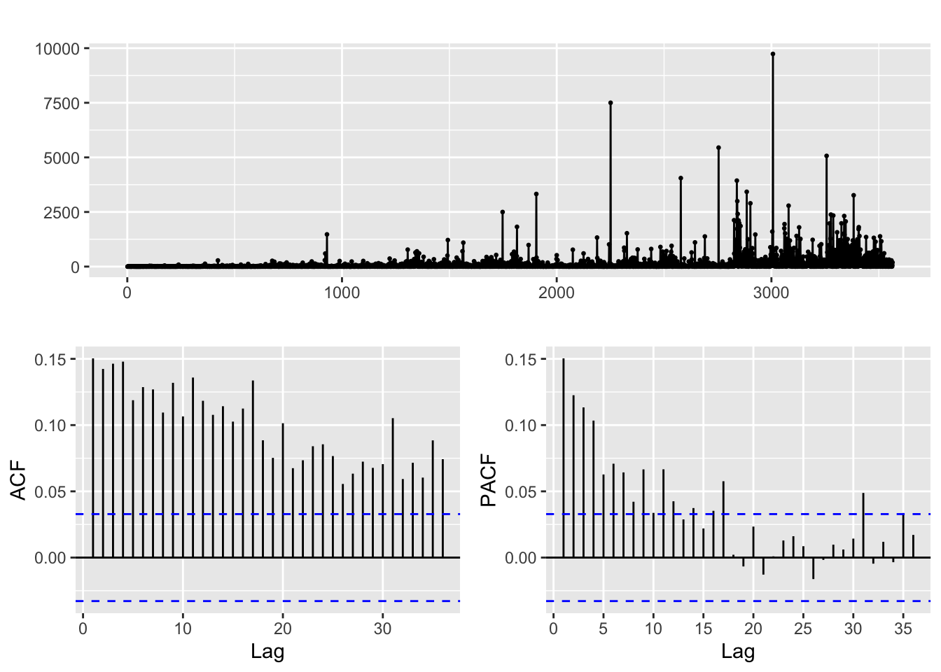

All the squared residuals plots show signs of volatility clustering. After conducting the model diagnostics and perusing the ACF and PACF of the squared residuals, a GARCH(p,q) model is suitable for all financial series.

Fitting GARCH(p,q) Models to Residuals

Lockheed Martin (LMT)

Code

model <- list() ## set counter
cc <- 1
for (p in 1:10) {
  for (q in 1:10) {
  
model[[cc]] <- garch(res.arima.lmt,order=c(q,p),trace=F)
cc <- cc + 1
}
} 

## get AIC values for model evaluation
GARCH_AIC <- sapply(model, AIC) 

model[[which(GARCH_AIC == min(GARCH_AIC))]] ## model with lowest AIC is the best and output model summary

Call:
garch(x = res.arima.lmt, order = c(q, p), trace = F)

Coefficient(s):
       a0         a1         b1  
3.503e-06  6.444e-02  9.227e-01  

Raytheon Technologies (RTX)

Code

model <- list() ## set counter
cc <- 1
for (p in 1:10) {
  for (q in 1:10) {
  
model[[cc]] <- garch(res.arima.rtx,order=c(q,p),trace=F)
cc <- cc + 1
}
} 

## get AIC values for model evaluation
GARCH_AIC <- sapply(model, AIC) 

model[[which(GARCH_AIC == min(GARCH_AIC))]] ## model with lowest AIC is the best and output model summary

Call:
garch(x = res.arima.rtx, order = c(q, p), trace = F)

Coefficient(s):
       a0         a1         a2         b1         b2         b3         b4  
1.148e-05  1.170e-01  9.930e-02  3.545e-01  1.293e-02  1.713e-02  6.380e-02  
       b5         b6  
1.396e-08  3.020e-01  

Dow Jones Travel and Tourism Index (DJUSTT)

Code

model <- list() ## set counter
cc <- 1
for (p in 1:20) {
  for (q in 1:20) {
  
model[[cc]] <- garch(res.arima.djustt,order=c(q,p),trace=F)
cc <- cc + 1
}
} 

## get AIC values for model evaluation
GARCH_AIC <- sapply(model, AIC) 

model[[which(GARCH_AIC == min(GARCH_AIC))]] ## model with lowest AIC is the best and output model summary

Call:
garch(x = res.arima.djustt, order = c(q, p), trace = F)

Coefficient(s):
       a0         a1         a2         a3         a4         a5         a6  
5.574e-03  5.902e-02  7.799e-02  1.116e-01  7.665e-02  5.615e-02  4.856e-02  
       a7         a8         a9        a10        a11        a12        a13  
1.679e-01  6.062e-02  1.043e-02  5.722e-02  4.919e-02  5.030e-02  8.140e-15  
      a14        a15        a16        a17         b1         b2         b3  
7.457e-02  2.864e-02  1.605e-01  1.063e-01  3.581e-02  3.671e-02  3.425e-02  

Lockheed Martin (LMT):

The outputted model is GARCH(1,1). Therefore, the final model is ARIMA(0,1,1) + GARCH(1,1)

Raytheon Technologies (RTX):

The outputted model is GARCH(2,6). Therefore, the final model is ARIMA(0,1,0) + GARCH(2,6)

Dow Jones Travel and Tourism Index (DJUSTT):

The outputted model is GARCH(17,3). Therefore, the final model is ARIMA(0,1,0) + GARCH(17,3)

Fitting ARIMA + GARCH (final model) and Conducting Box-Ljung Test on Residuals

Lockheed Martin (LMT)

Code

spec <- ugarchspec(variance.model = list(model = "sGARCH", garchOrder = c(1,1)), 
                   mean.model = list(armaOrder = c(0,1)), 
                   distribution.model = "std")

fit.lmt <- ugarchfit(spec, data = res.arima.lmt, solver = "hybrid")


# Perform Box-Ljung test on residuals
cat("Box-Ljung Test on Residuals based on lag = 1: \n")

Box-Ljung Test on Residuals based on lag = 1: 

Code

Box.test(fit.lmt@fit$residuals, type="Ljung-Box")

    Box-Ljung test

data:  fit.lmt@fit$residuals
X-squared = 1.4829, df = 1, p-value = 0.2233

Code

cat("\nBox-Ljung Test on Residuals based on lag = 10: \n")

Box-Ljung Test on Residuals based on lag = 10: 

Code

Box.test(fit.lmt@fit$residuals, type="Ljung-Box", lag=10) # not signif after lag = 11 

    Box-Ljung test

data:  fit.lmt@fit$residuals
X-squared = 11.642, df = 10, p-value = 0.3097

Raytheon Technologies (RTX)

Code

spec <- ugarchspec(variance.model = list(model = "sGARCH", garchOrder = c(2,6)), 
                   mean.model = list(armaOrder = c(0,1,0)), 
                   distribution.model = "std")

fit.rtx <- ugarchfit(spec, data = res.arima.rtx, solver = "hybrid")


# Perform Box-Ljung test (lag=1 and lag=10) on residuals
cat("Box-Ljung Test on Residuals based on lag = 1: \n")

Box-Ljung Test on Residuals based on lag = 1: 

Code

Box.test(fit.rtx@fit$residuals, type="Ljung-Box")

    Box-Ljung test

data:  fit.rtx@fit$residuals
X-squared = 0.0035968, df = 1, p-value = 0.9522

Code

cat("\nBox-Ljung Test on Residuals based on lag = 5: \n")

Box-Ljung Test on Residuals based on lag = 5: 

Code

Box.test(fit.rtx@fit$residuals, type="Ljung-Box", lag=5) # not signif after lag = 3

    Box-Ljung test

data:  fit.rtx@fit$residuals
X-squared = 15.563, df = 5, p-value = 0.008208

Dow Jones Travel and Tourism Index (DJUSTT)

Code

spec <- ugarchspec(variance.model = list(model = "sGARCH", garchOrder = c(3,9)), 
                   mean.model = list(armaOrder = c(0,1,0)), 
                   distribution.model = "std")

fit.djustt <- ugarchfit(spec, data = res.arima.djustt, solver = "hybrid")


# Perform Box-Ljung test (lag=1 and lag=10) on residuals
cat("Box-Ljung Test on Residuals based on lag = 1: \n")

Box-Ljung Test on Residuals based on lag = 1: 

Code

Box.test(fit.djustt@fit$residuals, type="Ljung-Box")

    Box-Ljung test

data:  fit.djustt@fit$residuals
X-squared = 0.011276, df = 1, p-value = 0.9154

Code

cat("\nBox-Ljung Test on Residuals based on lag = 5: \n")

Box-Ljung Test on Residuals based on lag = 5: 

Code

Box.test(fit.djustt@fit$residuals, type="Ljung-Box", lag=5) # not signif after lag = 5

    Box-Ljung test

data:  fit.djustt@fit$residuals
X-squared = 5.5925, df = 5, p-value = 0.3479

Lockheed Martin (LMT):

The Box-Ljung Test outputs a p-value > 0.05 for all lags up until 10, which signifies that the ARIMA(0,1,1) + GARCH(1,1), fitted on LMT, captures the autocorrelation structure in the data until lag 10. This indicates that the model is robust is forecasting the volatility of future returns of LMT.

Raytheon Technologies (RTX):

The Box-Ljung Test outputs a p-value > 0.05 for all lags up until 3, which signifies that the ARIMA(0,1,0) + GARCH(2,6), fitted on RTX, captures the autocorrelation structure in the data until lag 3. The model can still be employed to forecast the volatility of future returns of RTX and is a good indication that the model is capturing the important dynamics in the data.

Dow Jones Travel and Tourism Index (DJUSTT):

The Box-Ljung Test outputs a p-value > 0.05 for all lags up until 5, which signifies that the ARIMA(0,1,0) + GARCH(17,3), fitted on DJUSTT, captures the autocorrelation structure in the data until lag 3. The AR component of the GARCH model is significantly more complex than that of the other models because it has a much higher number of GARCH terms (17) relative to the other models.

Generally, a model with more parameters is considered more complex because it has more degrees of freedom to fit the data, which can lead to overfitting and poor out-of-sample performance. However, a more complex model may be necessary to adequately capture the dynamics of the DJUSTT, which has a relatively more complex and highly volatile time series. This can also be seen in its returns plot in the previous section.

Model Equations

Lockheed Martin (LMT):

ARIMA(0,1,1) + GARCH(1,1):

\(r_t = \phi r_{t-1} + \epsilon_t + \theta \epsilon_{t-1}\), where \(\phi\) and \(\theta\) are the autoregressive and moving average parameters, respectively, for the conditional mean of the time series, and \(\epsilon_t\) is a standardized white noise process with mean 0 and variance 1.

The conditional variance of the time series, \(\sigma_t^2\), is modeled as a GARCH(1,1) process as:

\(\sigma_t^2 = a_0 + \alpha_1 \epsilon_{t-1}^2 + \beta_1 \sigma_{t-1}^2\), where \(\alpha_1\) and \(\beta_1\) are the autoregressive and moving average parameters, respectively, for the squared residuals \(r_{t-1}^2\) and the conditional variances \(\sigma_{t-1}^2\). The parameter \(a_0\) represents the constant variance term.

Raytheon Technologies (RTX):

ARIMA(0,1,0) + GARCH(2,6): \(r_t = \phi r_{t-1} + \epsilon_t\), where \(\phi\) and \(\theta\) are the autoregressive and moving average parameters, respectively, for the conditional mean of the time series, and \(\epsilon_t\) is a standardized white noise process with mean 0 and variance 1.

The conditional variance of the time series, \(\sigma_t^2\), is still modeled as a GARCH(2,6) process as:

\(\sigma_t^2 = a_0 + \alpha_1 \epsilon_{t-1}^2 + \alpha_2 \epsilon_{t-2}^2 + \beta_1 \sigma_{t-1}^2 + \beta_2 \sigma_{t-2}^2 + \beta_3 \sigma_{t-3}^2 + \beta_4 \sigma_{t-4}^2 + \beta_5 \sigma_{t-5}^2 + \beta_6 \sigma_{t-6}^2\) , where \(\alpha\) and \(\beta\) are the autoregressive and moving average parameters, respectively, for the squared residuals \(r_{t-j}^2\) and the conditional variances \(\sigma_{t-j}^2\). The parameter \(a_0\) represents the constant variance term.

Dow Jones Travel and Tourism Index (DJUSTT):

ARIMA(0,1,0) + GARCH(17,3):

\(r_t = \phi r_{t-1} + \epsilon_t\), where \(\phi\) is the autoregressive parameter for the conditional mean of the time series, and \(\epsilon_t\) is a standardized white noise process with mean 0 and variance \(\sigma_t^2\).

The conditional variance of the time series, \(\sigma_t^2\), is modeled as a GARCH(17,3) process as:

\(\sigma_t^2 = a_0 + \sum_{i=1}^{17} \alpha_i \epsilon_{t-i}^2 + \sum_{j=1}^{3} \beta_j \sigma_{t-j}^2\), where \(\alpha_i\) and \(\beta_j\) are the autoregressive and moving average parameters, respectively, for the squared residuals \(r_{t-i}^2\) and the conditional variances \(\sigma_{t-j}^2\). The parameter \(a_0\) represents the constant variance term.

Volatility Plots for ARIMA + GARCH Models

These plots represent the estimated conditional variances of the ARIMA residuals obtained from the fitted sGARCH model. The y-axis shows the values of the estimated variances, while the x-axis represents the time period for which the variances were estimated.

Lockheed Martin (LMT)

Code

hhat <- (fit.lmt@fit$sigma^2)
plot.ts(hhat, col="#005BAD")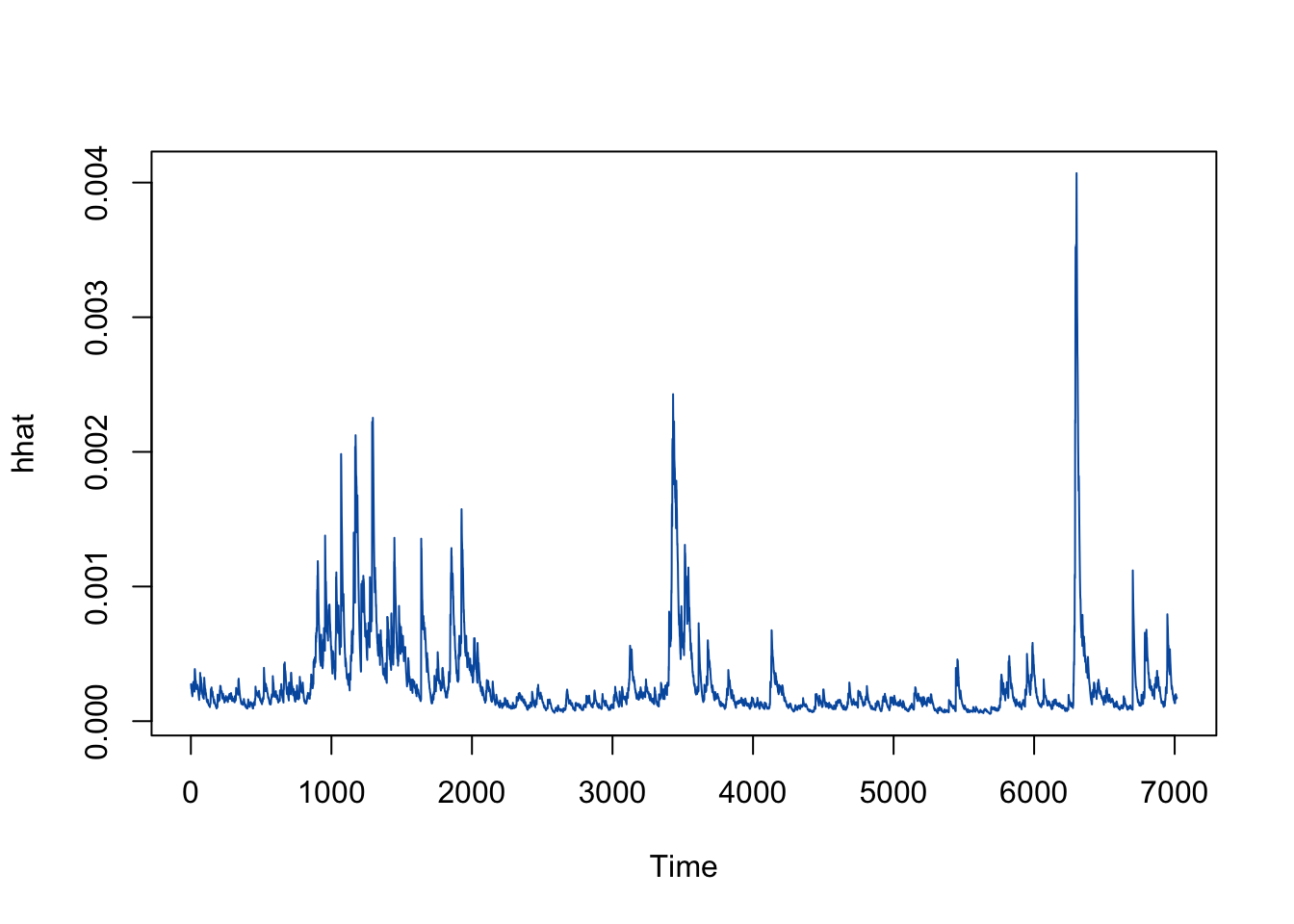

Raytheon Technologies (RTX)

Code

hhat <- (fit.rtx@fit$sigma^2)
plot.ts(hhat, col="#E61231")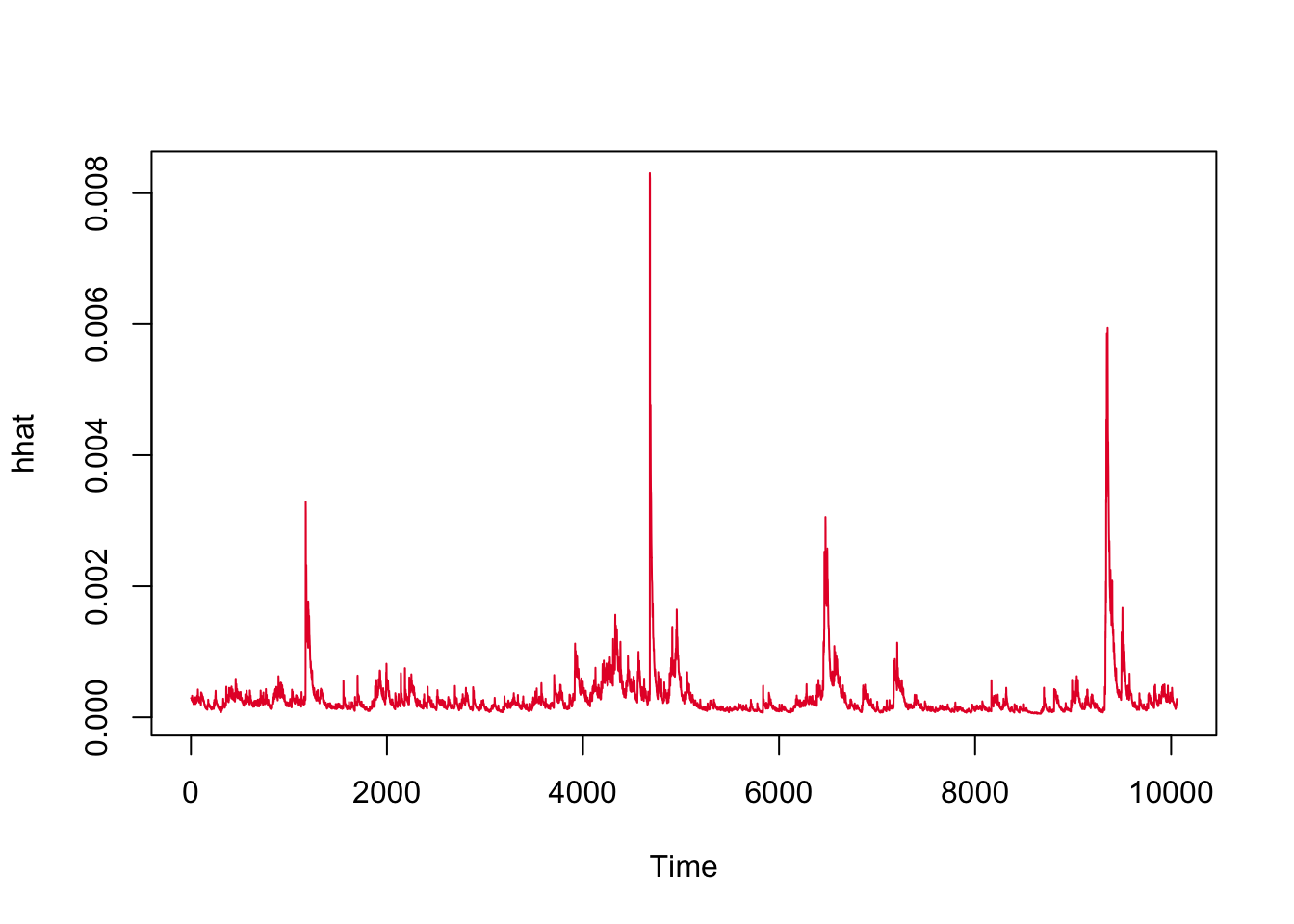

Dow Jones Travel and Tourism Index (DJUSTT)

Code

hhat <- (fit.djustt@fit$sigma^2)
plot.ts(hhat)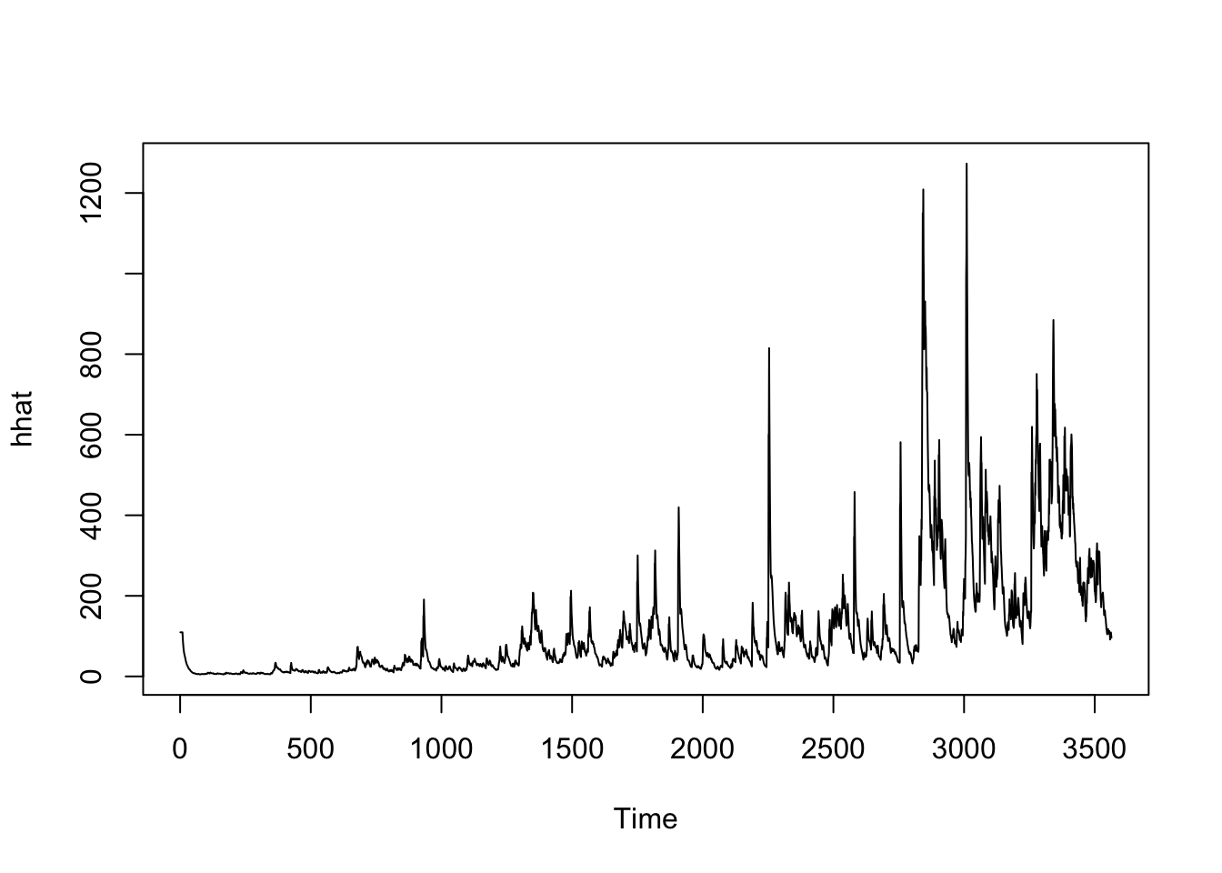

Lockheed Martin (LMT):

The volatility plot provides evidence that LMT’s stock price experienced relatively higher volatility in the following periods: end of 1998 to beginning of 2003, the beginning of the 2008 financial crisis, and the onset of the COVID-19 pandemic.

Raytheon Technologies (RTX):

The volatility plot provides evidence that RTX’s stock price experienced relatively higher volatility in the following periods: end of 1987 to beginning of 1988 (signifying that the Black Monday stock market crash catalyzed RTX’s lowest stock price until 2019), quickly after the 9/11 attacks, the beginning of the 2008 financial crisis, and the onset of the COVID-19 pandemic. A key finding here is that military targets were highest in 1986 due to The Macheteros, a clandestine militant and insurgent organization based in Puerto Rico, claiming responsibility for bombing U.S. armed forces facilities. Coupled with this attack and Black Monday, the 1983 Kuwait bombings could also provide some explanation to RTX’s stock being high volatility around 1987 as their employees were targeted but none injured due to failed bombings.

Dow Jones Travel and Tourism Index (DJUSTT):

The volatility plot provides evidence that RTX’s stock price experienced relatively higher volatility in the following periods: President Trump’s Travel Ban in October 2017 and the onset of the COVID-19 pandemic. The index is fairly new new compared to the other 2 stocks and, hence, its higher volatility is warranted, especially due to the COVID-19 pandemic.

Section Code

Code for this section can be found here